We have now practiced formulation, visual evidence, writing, optimization, changing systems, forecasting, data cleaning, regression, clustering, and evaluation. A competition prompt can ask for several of them at once. If you and two teammates have only three days, where do you begin and when do you stop improving one module? That is the question for our studio lesson.

We will choose a problem with accessible evidence, build a small complete baseline, map dependencies between modules, and reserve time for tests and writing. The mock cases include robot localization and decisions under noisy information; they are vehicles for practicing the whole workflow, not reasons to use a complicated method automatically. Think of this as our rehearsal: I will ask what result the team can defend at each stage and what failure it still needs to investigate.

Competition performance is a systems problem. Modeling, coding, writing, and verification must advance together, because a brilliant result that cannot be explained or reproduced is not a complete submission.

Select a problem with evidence

During the first pass, every teammate independently records required outputs, available data, plausible baselines, major risks, validation opportunities, and a possible distinctive contribution.

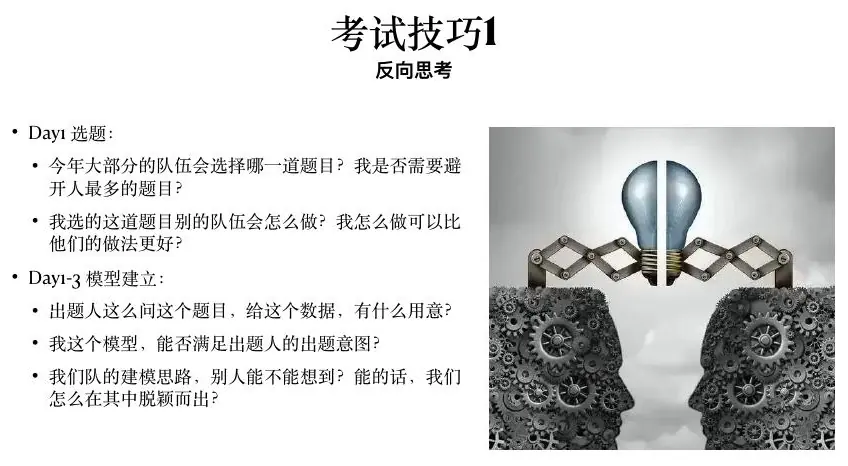
Choose the problem whose key mechanism the team can defend—not the one with the most familiar buzzwords. Ask how many teams may use the obvious method and identify a meaningful improvement grounded in the problem.

Create a requirement table with one row per question. For each row list output, model, data, figure, validation, and current status. This table is the team’s control panel.

A prompt that looks larger than it is

Imagine receiving a competition prompt about heat risk in a city. It provides daily temperature observations, a map of population by district, limited information about tree cover and cooling centers, and a budget for interventions. It asks the team to identify vulnerable areas, estimate future heat exposure, propose where to spend money, and discuss uncertainty. One teammate sees a forecasting problem, another sees an optimization problem, and the third sees a mapping problem. All three are right, but if they work in isolation they may produce incompatible answers. The forecast must refer to the same districts and time horizon as the allocation; the vulnerability measure must refer to people the interventions actually help.

We can make the prompt manageable by naming its outputs in order. First, a district-year table with consistent units and data dates. Second, a risk measure for each district that distinguishes hazard from vulnerability. Third, a forecast or scenario for future heat, with a comparison to a simple baseline. Fourth, a feasible intervention plan under the stated budget. Fifth, a test of what changes when temperature, costs, or benefit assumptions move. These are not five independent essays. The first output supplies the second; the second and third supply the fourth; the fifth checks the fourth.

Choose an observational unit early. Is a row one weather station-day, one district-day, or one district-year? Temperature is measured by stations; residents are counted by district; intervention spending is decided by district. We might summarize station readings into district-day heat exposure, then aggregate appropriately for the decision horizon. If we attach the same district population to every hourly station reading and later sum population, we can accidentally count people many times. That is a join error with policy consequences.

The word “vulnerable” needs an operational definition. Heat risk can increase with exposure, age, medical conditions, housing quality, and lack of cooling access. The provided population table may only offer total residents. Do not invent a precise health-risk estimate from that total. We can construct a proxy and call it a proxy, note missing age or housing information, and test whether plausible vulnerability ranges change the proposed plan. A modest model that names its missing mechanism is more defensible than a sophisticated score whose interpretation is hidden.

The team also has to read constraints carefully. A 6-million-dollar budget means we cannot fund every project. A cooling center needs an accessible building and staff; planting trees may have delayed effects and depend on water. If the prompt asks for actions this summer, a new tree canopy cannot be credited with immediate full cooling. Time order is a model constraint, not a sentence to add in limitations after the recommendation is calculated.

The team should write a provisional decision sentence: “Allocate up to 6 million across feasible district interventions to reduce expected person-days above a heat-risk threshold next summer, while maintaining access to at least one cooling site in each high-risk district.” The threshold and costs will come from the prompt or be declared assumptions. The sentence aligns data, forecast, evaluation, and optimization around one action.

There may be a more attractive competition choice: a robotics prompt with beautiful diagrams or a market prompt with a rich dataset. The same test applies. Can we define the requested output, locate usable evidence, produce a baseline, and check a result? A topic that sounds exciting but lacks measurable constraints or available data may be harder to defend. Problem selection is not a popularity contest among algorithms; it is a judgment about which mechanism the team can explain under the actual deadline.

Choosing a competition problem is not the end of formulation. We need a complete, checkable first answer before a complex graph, market, or simulation model can earn its place. That baseline is the reference for every improvement that follows.

Build a baseline first

During the first modeling block, produce a complete but simple chain from raw data to one answer. This baseline becomes a test harness for every extension. Save its metrics and figures.

Maintain a decision log containing assumptions, parameter sources, rejected approaches, and reasons. Use version control or timestamped archives. Record random seeds and environments. An improvement should be accepted only after it beats the baseline under the same evaluation.

A three-district baseline we can check

Continue the invented heat case. Let North, Central, and South have populations 1,000, 800, and 1,200. Suppose a baseline scenario estimates 12, 8, and 10 dangerous-heat days next summer. A deliberately simple exposure proxy is population times dangerous days: 12,000, 6,400, and 12,000 person-days. North and South tie on this proxy, while Central is lower. We can calculate each number by hand, so if a later pipeline reports 120,000 for North, we know to inspect a factor of ten, a duplicate join, or an incorrect unit.

This proxy is not expected illness. It assumes every person experiences every district heat day and does not adjust for indoor cooling, hours outside, age, or neighborhood temperature differences. Its value is that it has clear units and a visible limitation. We can ask whether data on vulnerable residents or cooling access are available. If not, define a multiplier scenario rather than pretending the factors are known. South may have a hypothetical vulnerability multiplier of 1.3 and North 1.0; their adjusted proxies become 15,600 and 12,000. This shows how an unmeasured social factor could change priorities, but the multiplier must be labeled as a scenario, not a measured fact.

Suppose each district has one intervention candidate. North’s center expansion costs 2 million and is estimated to avoid 3,000 risky person-days; Central’s shaded bus stops cost 1 million and avoid 1,000; South’s building retrofit costs 4 million and avoids 5,000. These are invented classroom estimates. With a 6-million budget, North plus South exactly fits and yields 8,000 avoided person-days; North plus Central costs 3 and yields 4,000; Central plus South costs 5 and yields 6,000. If projects do not overlap and benefits are additive, North plus South is the baseline plan. If the prompt also requires a cooling site in Central, that plan violates a hard service rule and the candidate set needs redesign.

The arithmetic is transparent. Define a binary decision variablefor each project and maximizesubject to. Enumerating eight possible combinations by hand verifies the optimizer on this tiny case. The larger dataset may need a solver, but if the solver cannot reproduce the toy optimum, the problem is likely in our coefficients, units, or constraints rather than in the city.

Now ask whether the apparent optimum is trustworthy. Benefits are estimated, not observed, and might interact. A retrofit in South and a cooling center in North serve different people, so additivity may be plausible. If two interventions are in the same district, their effects may overlap; adding them could double-count avoided exposure. Costs might include operations beyond capital spending. Budget horizon and benefit horizon must match. A project that takes two years to complete cannot be credited with full next-summer benefit. A simple baseline is credible when its assumptions can be tested.

When an extension is proposed, measure its value against the baseline. A sophisticated weather model might improve forecasts, but does it change which projects fit the budget? A refined vulnerability map might move the South intervention to another block. A robust optimizer might sacrifice 500 nominal avoided person-days but perform better under hotter scenarios. Each upgrade must answer a visible failure, not simply add complexity to the paper.

The complete chain is possible already: observations become exposure proxies; proxies and intervention estimates become a feasible plan; scenarios test whether it holds; a recommendation describes the action and its limits. We do not need to wait for an advanced technique to start the manuscript. Drafting the first result now helps reveal which requested output our chain still cannot answer.

Case pattern: graph-based estimation

The first simulation material illustrates a reusable pattern. Unknown node states are connected by noisy relative measurements. Define residualon each edge and minimize

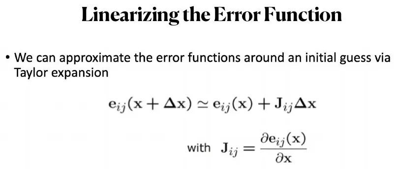
Linearization near the current estimate yields

Each residual touches only a few node states, so the Jacobianand approximate Hessianare sparse. The lesson is broader than robotics: exploit locality and sparsity instead of passing a structured problem to a dense black box. Fix a reference node or prior to remove gauge ambiguity, then inspect residuals after optimization.

Walk a loop before building a matrix

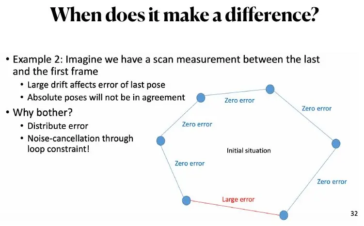
Picture a robot traveling along a hallway in three legs and returning to its starting point. It measures each displacement with a wheel encoder. If the true steps are +1 meter, +1 meter, and −2 meters, they sum to zero and the robot closes the loop. Noisy measurements might instead read +1.1, +0.9, and −1.9 meters. Adding them gives +0.1 meter. The robot’s integrated estimate ends ten centimeters from its start even though it physically returned. That ten-centimeter gap is a concrete residual, not an aesthetic imperfection in a plot.

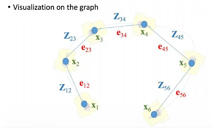
An obvious but incomplete “fix” is to drag the last plotted point back to the beginning. It closes the visible loop without asking which measurement was wrong, and it can distort distances along earlier edges. A graph formulation represents the three unknown positions as nodes and the noisy measured displacements as edges. Each edge predicts a differenceand compares it with its measurement. In one dimension a residual is. Minimize the weighted sum of squared residuals, withas the reference origin.

For equal confidence in the three measurements, we can understand the least-squares adjustment by hand. The three measured displacements sum to +0.1 but a closed loop must sum to zero. Distribute a total correction of −0.1 evenly: each corrected displacement changes by −0.1/3≈−0.0333. They become about 1.0667, 0.8667, and −1.9333; the sum is zero. The corresponding positions are,,, and then back to. Each edge takes a small residual rather than forcing one edge to absorb the whole contradiction.

Equal distribution depends on equal uncertainty. If the first two measurements are precise and the third comes from a shaky visual loop-closure detector, the optimization should trust the first two more and adjust the third more. The information matrixis related to inverse measurement covariance: a high-confidence edge receives stronger penalty for a given residual. A robot paper that writes a weighted objective without explaining where edge confidence came from has hidden a consequential assumption. A false loop closure can pull an entire map out of shape if given unjustified high weight.

We have also seen why fixing a pose is necessary. Relative displacements tell us the shape of the path, but not its absolute coordinate. Add 100 meters to everyand every differencestays the same. Without a fixed reference or prior, the normal equations have a free translation direction, called gauge freedom. In 2D or 3D pose graphs, global rotation can also be unconstrained. An optimizer reporting a singular matrix may be revealing this missing reference, not failing because its numerical method is weak.

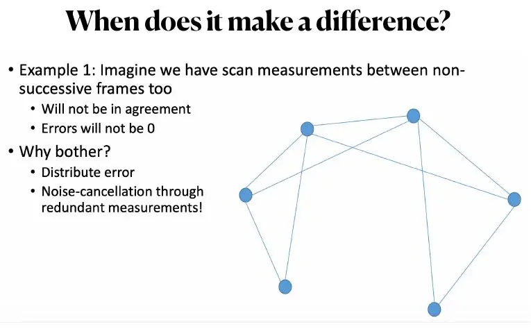
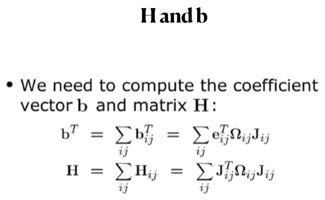
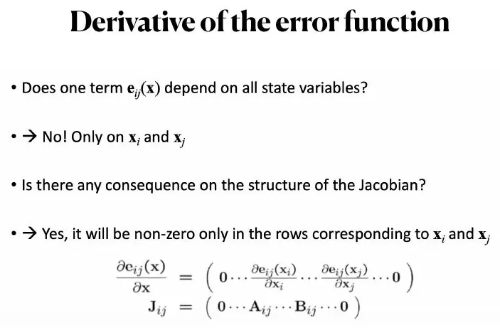
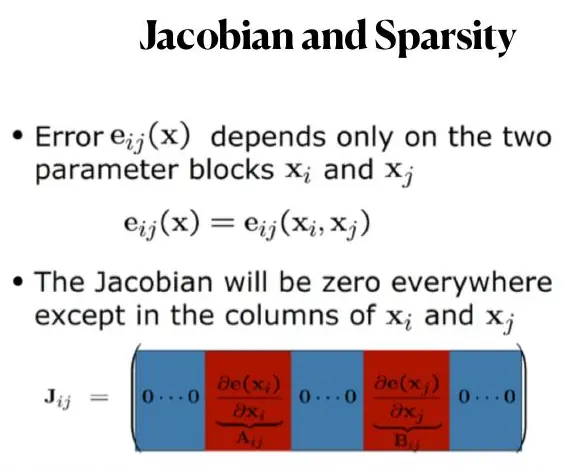
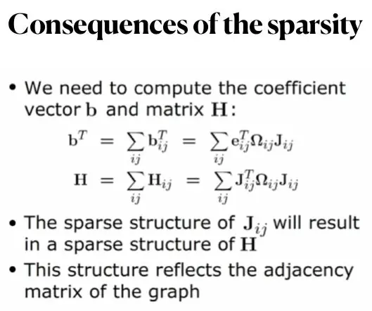
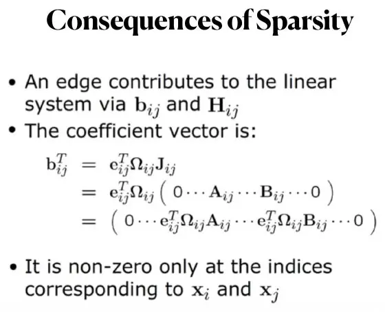
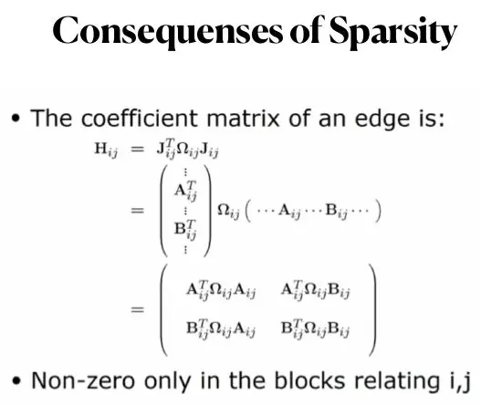
Sparsity comes directly from the story. The edge connecting nodes 1 and 2 depends on those two positions, not on every other position in a thousand-node route. Its Jacobian row has nonzero entries only in the columns for its incident nodes. The normal matrix couples neighboring states, with extra off-diagonal blocks where loop-closure edges connect distant times. A dense array ignores that locality and wastes memory. The graph drawing is therefore more than an illustration: it tells us the nonzero pattern of the computation.

After optimization, do not celebrate only the lower total cost. Examine residuals by edge. If nearly all wheel-encoder edges have small errors but one visual loop closure has a huge one, ask whether that closure matches the same physical place. A robust loss can reduce the influence of an outlier, but it should follow diagnostic evidence. Downweighting every inconvenient residual to make a smooth picture would hide a faulty model or sensor.

This graph example belongs in a modeling studio because it forces several course habits to work together. We formulate a physical consistency rule; calculate a tiny baseline by hand; assign units and uncertainty; use sparse numerical structure; and inspect residuals before making a claim. The same pattern appears outside robotics when noisy relative observations link locations, times, or entities. We can now see what a “graph model” contributes instead of treating the phrase as a fashionable label.

Case pattern: noisy markets and decisions

The second simulation material combines bid–ask data, relative spreads, liquidity, dependence, risk, and allocation. A reusable workflow is:

1. define every order-book feature with unit and timestamp;
2. separate cross-sectional dependence from temporal dependence;
3. estimate return and liquidity risk without future leakage;
4. optimize allocation under capital and execution constraints;
5. stress-test fees, slippage, and regime change.

Midprice isand spread is, whereandare best ask and bid. Relative spread divides by midprice for comparability. A backtest is invalid if decisions at timeuse a quote, return, or aggregate that became known later.

The price you can trade is not the price you plot

Suppose an order book quotes a best bid of USD 99.80 and best ask of USD 100.20 for one share. The midprice is USD 100.00, the quoted spread is USD 0.40, and the relative spread is. A chart may show a neat USD 100.00 “price,” but a buyer crossing the spread pays USD 100.20, while a seller crossing it receives USD 99.80. If a strategy buys and immediately sells without the market moving, it loses USD 0.40 per share before fees. A backtest that buys at mid and sells at mid invents a free execution that the order book did not offer.

Now imagine that the midprice rises to USD 100.30 one minute later, with bid USD 100.10 and ask USD 100.50. A simplistic paper profit is USD 0.30 for buying at the first mid and selling at the second mid. The actually executable round trip—buy at USD 100.20 and sell at USD 100.10—loses USD 0.10 before fees. This is why execution assumptions belong inside the decision model, not in a cautionary final sentence. A strategy that looks promising on midprice returns may be unprofitable after spread, slippage, and limited depth.

Depth matters because a quoted best ask may cover only a few shares. If the order wants 1,000 shares, later levels in the book may be more expensive. The average execution price depends on order size and liquidity; using the first ask for the entire order can overstate profit. A simple baseline can cap trade size at available top-of-book depth and compare it with a more detailed order-book simulation. The upgrade is justified if it changes the allocation or reported performance.

Be precise with timestamps. A quote at 10:00:00, a decision at 10:00:01, and a trade at 10:00:02 have a clear information order. A five-minute return ending at 10:05 cannot be used as a 10:00 feature. A daily closing volume may be known only after trading ends, so it cannot inform an intraday action made earlier. Aggregating a time series before splitting train and test can accidentally leak later statistics into earlier features. The question is always, “Could the decision maker have known this number then?”

Cross-sectional dependence means instruments move together at the same time; temporal dependence means one instrument’s earlier values help predict later values. A heat map of correlations between assets describes the first, while an autocorrelation plot describes the second. A high correlation might reflect common exposure to a market factor rather than a stable pairwise trading relation. If the regime changes, both patterns can change. Forecasting a return, estimating a covariance, and choosing an allocation are separate modules; using one method for all three because it has a popular name obscures the roles.

Consider a decision to allocate capital between two assets. A forecast may say asset X has higher expected return, but its quoted spread is wider and its volatility is much larger. The objective should use net expected return after execution cost and a risk term with clearly stated units. Add a capital constraint, a position-size limit, and perhaps a liquidity limit. If the solution assumes we can instantly buy more than the book supplies, it is infeasible even if the optimization routine reports “success.”

Backtest the decision chronologically. Establish a simple baseline such as holding cash or a fixed allocation, and compare strategies under the same starting capital, transaction-cost rule, and trading times. Report not only average return but drawdown, turnover, and performance during stressed periods. A model can outperform during calm weeks yet fail when spreads widen precisely as the decision becomes most consequential. One favorable historical period is evidence of what happened there, not a promise about future markets.

This market example is technically different from the robot loop, but it tests the same intellectual discipline. The graph case asks whether measured relations can be reconciled without hiding a bad edge. The market case asks whether an apparently profitable relation survives feasible execution and information timing. Both require a small checkable calculation before a large algorithm. The nicest code is not a substitute for a physical or operational reality check.

The graph and market patterns show technical possibilities. Under a three-day deadline, the decisive question becomes who tests each part, who writes the explanation, and how everyone sees the same current version.

Team operating rhythm

Use short synchronization cycles. At each checkpoint confirm the current answer to every subproblem, unresolved assumptions, reproducible figures, experiments still worth their time, and the next integration deadline.

One person owns the master manuscript, but all teammates review equations, code outputs, and claims. Use notebooks for exploration, then consolidate the final pipeline so it runs from a clean state. Split long programs into testable stages rather than debugging one monolith.

Three people, one result

Consider three teammates working on our heat problem. Ada audits temperatures and population, Ben builds the intervention model, and Chen writes the report and validation code. If Ada produces district daily maxima but Ben expects annual counts of days above a threshold, their interface is not merely a filename. They need to agree on what each row means, the threshold, units, geography, and date. A shared district-year table with a data dictionary is an interface contract between their modules.

Suppose Ada discovers that South’s temperature station was moved midway through the record. The forecast module may change its inputs, the estimated heat days may change, the intervention benefits may change, and the paper’s headline recommendation may change. If these outputs live in three manually edited spreadsheets, the team can accidentally submit a forecast from the corrected data and a project plan from the old data. The better arrangement is a repeatable sequence: raw files remain untouched; a documented cleaning step creates the aligned district table; forecast and allocation scripts read that table; result tables and figures are regenerated from the same run.

Ben may find that the exact optimizer chooses North plus South, while Chen’s summary says “North and Central” because a provisional draft was not updated. This is a common failure: the computation is right, but the manuscript is stale. Store headline results in a small machine-readable output table with the chosen project IDs, total cost, objective value, and scenario name. When writing, compare every claim in prose with that table. A cold-reading teammate should be able to locate the same chosen projects in the figure, table, and code output.

Version control helps here if used calmly. Each teammate can work on a named module, commit small understandable changes, and review the integration. A giant merge of three independent final notebooks near the deadline is risky because assumptions may differ even when code merges cleanly. Pair-review the interface early. If a change alters the observational unit, everyone downstream needs to know; if it only changes a plot’s color, the model outputs should stay the same. Communicating that distinction saves real debugging time.

Exploration notebooks are useful for learning the data, but a notebook can silently depend on cells run out of order. Before making the final claim, rerun it from a clean state. Better yet, consolidate stable transformations into a script or functions with declared inputs. Record a random seed for simulation and any model split, but do not mistake a seed for reproducibility if the raw data, package versions, or manual preprocessing steps are missing.

Cross-review is intellectual, not merely stylistic. Ada should ask Ben why a retrofit affects all of South if it only covers selected buildings. Ben should ask Ada how a station move was handled. Chen should ask both how the recommendation behaves if South’s benefit estimate falls. Every teammate should be able to explain the main decision sentence and one central limitation. If only the specialist understands a module, the paper may contain a gap nobody else can see.

A useful team meeting is centered on one current table, not on reports of hours worked. Show the latest district exposures, project coefficients, feasible combinations, and held-out forecast errors. Ask which number is provisional, which is verified, and which choice depends on it. That conversation leads to decisions: collect a missing source, revise a coefficient, keep the baseline, or freeze a module. It is the practical meaning of “integrate continuously.”

Keep the stages connected

• Opening: interpret and choose; build data audit and baseline.
• Middle: develop the central model; validate continuously; begin final figures.
• Closing: freeze the model early enough to write, audit, reproduce, and submit.

Do not let every teammate browse outside solutions. Assign one person to monitor useful references while the others preserve independent reasoning. Use AI as an assistant for explanation, debugging, and alternatives only when the team can verify every equation, citation, and line of code.

Write while modeling

Create the paper structure early: restatement, analysis, assumptions, notation, models, results, validation, strengths and limitations, conclusion, references, and appendix. Insert figures and quantitative results as soon as they stabilize. Write the abstract last.

Use scientific language, consistent symbols, numbered key equations, captions below figures, titles above tables, and citations at the point of use. Open questions must become either completed analyses or explicit limitations before submission.

Write the result before writing the abstract

Imagine a draft sentence: “Our proposed plan is robust and dramatically lowers heat risk.” It sounds decisive, but it has no quantitative anchor or operating range. Replace it with the invented teaching result: “Under the 6-million budget and the stated intervention-benefit estimates, funding North and South avoids 8,000 modeled risky person-days; the choice must be revisited if South’s efficacy or Central’s cooling-access rule changes.” This sentence is longer but far more informative. It names the action, unit, model status, assumption, and condition.

The methods section should let a curious reader reconstruct that sentence. It should say how station readings became dangerous-day estimates, why population times days was used as a proxy, how project benefits were estimated, and what binary budget program was solved. Do not simply list “ARIMA, TOPSIS, integer programming” in a paragraph. Each named technique needs a purpose and an output that feeds the next module. If a technique never changes or explains the recommendation, it may belong in a comparison or appendix rather than the main story.

For the first figure, show the original district exposure and the aligned threshold with units. For the second, show project options and budget feasibility, perhaps in a small table rather than a complicated visualization. For the third, show how the chosen portfolio changes under plausible benefit or cost scenarios. These figures each support a different claim: evidence, decision, robustness. A large gallery of decorative plots would not compensate for the absence of a direct answer.

Symbols must remain stable. Ifdenotes dangerous heat days for district, do not reusefor the Hessian in a heat-case equation without explanation. Ifis the intervention decision, declare whether it is binary, continuous spending, or an intensity. A constraint likeshould be read aloud: “The total cost of chosen projects cannot exceed the budget.” That spoken translation is a quick way to catch a coefficient in the wrong unit.

Write the abstract after results and limitations settle. An early abstract can accidentally promise a model that was abandoned or cite a result from a previous run. A final abstract can briefly state the question, the baseline, the justified extension, one check, and the conditional recommendation. It is a compressed version of the paper’s actual argument, not a promotional blurb.

If the model makes a novel contribution, describe it specifically. “We introduced a spatially overlapping intervention-benefit constraint and found it changed the selected sites under high-demand scenarios” is testable. “We developed an innovative comprehensive framework” says almost nothing. The competition paper is still a lesson to its reader: it should show what the mechanism is, why that mechanism matters, and how the evidence supports the action.

Final audit

Before submission:

• answer every requested question explicitly;
• verify anonymity and required file format;
• regenerate all numbers and figures;
• check units, symbols, references, and captions;
• include source code and necessary supporting data;
• test the archive on a clean machine;
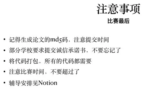
• generate any required checksum;
• submit early enough to recover from upload failure.

COMAP’s official instructions frame modeling, problem solving, writing, teamwork, and compliance as one integrated activity (MCM/ICM instructions ). The final report and supporting material are the executable record of the entire modeling process.

Verify a claim where it could fail

Before submission, the team should choose a few central claims and try to break them. For our heat plan, one claim is “North plus South is the best feasible portfolio under the nominal coefficients.” Verify the total cost, then enumerate every feasible combination in the three-project teaching case. If a solver output differs, inspect the input coefficients or the inequality direction. This hand check does not validate the real project’s benefit estimates, but it validates the arithmetic and program structure on a known small instance.

A second claim is “The forecast improves on a baseline.” Test it on years that were not used to fit either method, keeping the temperature threshold and district mapping fixed. If data preprocessing changes between methods, the comparison is unfair. Report the metric in days and connect it to the project choice. A one-day improvement in MAE could be useful or irrelevant, depending on whether it changes risk tiers or the selected projects. A statement of improved forecasting should not stand alone when the prompt asks for an intervention.

A third claim is “The recommended plan is robust.” Specify the range that makes this statement true. Maybe North plus South remains selected for South retrofit benefits between 4,500 and 5,000 risky person-days but changes below 4,000. That is a boundary, not an embarrassment. The reader learns which efficacy estimate deserves field verification. If a 10% cost increase makes the plan exceed budget, the nominal optimum is not financially robust even if exposure forecasts remain stable.

In the pose-graph case, a central claim may be “Global optimization closes the loop without distorting accurate measurements.” Test a three-node loop with known ground truth, add controlled noise, and compare edge residuals before and after optimization. Keep a fixed gauge. If a purported improvement comes only from reassigning the global origin, the geometry has not improved. Then insert one false loop closure and see whether the robust-loss variant prevents it from dragging every node. This gives the method an observed reason to exist.

In the market case, “The strategy earns positive net return” must be evaluated with feasible bid–ask execution and chronological information. Recalculate at least one trade manually, as we did with the USD 0.10 loss despite a rising midprice. Test spread widening, lower order-book depth, and a later market regime. If the strategy’s gain vanishes under realistic trading cost, do not bury that result behind a high gross-return chart.

These examples make validation specific. A generic statement “we conducted sensitivity analysis” is weaker than “the chosen portfolio changes when South’s retrofit benefit falls below this level.” A generic “the optimizer converged” is weaker than a manual loop check and residual inspection. A generic “backtest performance was strong” is weaker than a net-of-cost chronological comparison with a simple baseline. The final paper should make the checking mechanism visible beside each claim.

Reproducibility has an equally concrete meaning. A teammate opens a fresh copy of the input files, executes the declared pipeline, and gets the same chosen projects, scores, tables, and figures. They should not need to ask which notebook cell was run first or which spreadsheet column was edited by hand. A software version, random seed, data source, and transformation rule are useful because they make that independent run possible. They are not bureaucratic decorations in an appendix.

Compliance is a separate hard constraint. Even an excellent model may fail submission requirements if the final file format, anonymity, naming, or supporting materials are wrong. The team must check current official instructions rather than rely on an old template. The citation above identifies the kind of authoritative source to consult; competition rules can change. An early test upload, where the platform allows it, reduces the chance that a final-minute technical failure erases the work.

The final audit checks the submission. To prepare for the next problem, we should step back and ask which habits appeared in every case: formulation, units, baseline, validation, sensitivity, and communication.

Course synthesis

The reusable loop is

When time is short, simplify within this loop; do not skip the loop. A transparent, validated model that fully answers the prompt is stronger than a sophisticated algorithm disconnected from the decision.

Revisit the heat project as one connected argument

Use a generic urban heat-resilience problem: identify vulnerable locations, forecast future heat exposure, allocate a limited intervention budget, and explain how the plan changes under climate uncertainty. This case can combine the course without forcing every technique into one paper.

We have already calculated a three-district baseline. Let us examine what the real pipeline would need before turning those figures into a public plan. We start with temperatures. Suppose two sensors report daily maximum temperature near North: one in a shaded park and one beside a wide road. If the park station reads 33°C and the road station 37°C on the same day, a naive average is 35°C. But which temperature represents exposure for residents? The road station may be closer to a bus corridor; the park station may better represent a different block. The choice of aggregation depends on the decision and the spatial distribution of people. We can preserve both stations, map them, and test whether the North priority changes under alternative exposure assignments.

Timestamp semantics matter here too. A “daily maximum” for one station may be measured over midnight-to-midnight local time, while another source uses a 24-hour window ending at 08:00. Comparing their days without alignment can misclassify a heat event. The time-series lesson taught us to inspect frequency, time zone, missingness, and leakage before forecasting. A city intervention decided in spring cannot use heat observations from the following summer to construct its predictors, even if the full dataset is available when writing the paper.

For a baseline forecast, use a seasonal naive estimate or a recent-year heat-day average rather than immediately fitting a neural network. If North recorded 10, 13, and 12 dangerous days in the three previous summers, a three-year average of about 11.7 gives a checkable forecast of roughly 12 days. The arithmetic is trivial, but the uncertainty is not: three summers are sparse evidence, and a warming trend or unusual wildfire year could matter. Compare any advanced forecast to the baseline on earlier held-out summers, using the same threshold definition and district aggregation. If the advanced method cannot improve decision-relevant error, it need not appear in the final plan.

What is decision-relevant error? Underpredicting a severe heat season may leave cooling centers understaffed; overpredicting may consume scarce budget. MAE in days is understandable, but a policy paper should also examine whether forecast errors change the selected intervention. A forecast that is off by one day everywhere may leave the district ordering unchanged; a forecast that misses a localized three-day heat wave in South could reverse it. We can compare plans generated from forecasts with plans evaluated under observed historical heat. This connects prediction accuracy to action, rather than treating a forecasting leaderboard as the final objective.

Population data have their own limitations. Census residents are not the same as people present during a heat day. Commuters, students, tourists, and outdoor workers move across district boundaries. A person-days proxy based on resident count can be a starting point, but the intervention question may require daytime exposure. If the prompt lacks mobility data, say so and test a plausible range. If a bus-stop shade project targets commuters who do not live in Central, attributing its benefit only to Central residents is inconsistent. That mismatch should prompt a better beneficiary definition, not a more elaborate optimizer.

We might incorporate vulnerability as a dimension, but adding indicators without checking direction is dangerous. Older-adult share is often a risk proxy; tree cover may reduce heat exposure; air-conditioning access may reduce indoor risk but correlate with income; distance to a cooling center may become worse when the distance is larger. Entropy weights on those columns would reward variation, not necessarily protection of the most vulnerable. AHP could record city priorities, but whose priorities? The evaluation-model lesson taught us to state the value choice and to separate minimum service requirements from compensatory scores.

Once interventions are estimated, validate their benefit model. A shaded bus stop might reduce direct sun exposure at a specific location; it does not necessarily reduce all district heat-day person-counts. A building retrofit may reduce indoor heat for its occupants, not for everyone in the census district. Define each project’s target population and unit of benefit. If benefits are expressed in “risky person-days avoided,” show the physical or empirical path from the intervention to that quantity. When the path relies on an assumed efficacy, report the range and test the allocation over it.

Suppose South’s retrofit benefit could be anywhere from 3,500 to 5,000 person-days, and North’s center expansion from 2,500 to 3,000. North plus South still avoids between 6,000 and 8,000 under independent bounds; Central plus South avoids between 4,500 and 6,000 if Central remains at 1,000. At the shared boundary of 6,000 the choices may tie on benefit, and other criteria like coverage or cost become consequential. The interval does not need to be interpreted as a probability. It tells us where a plan could change and which efficacy measurement would be useful.

Our original binary program assumed one project per district. A real plan may include several sites, capacity limits, and travel distances. A cooling center serving two nearby districts can create overlapping benefits; a shaded route can help residents in multiple districts. A graph of access or a coverage model may be warranted when this interaction is measurable. But first check whether it changes the chosen plan relative to the district-level baseline. If not, the more complex network model may be valuable for implementation details rather than for the headline recommendation.

The paper should not claim that the baseline’s 8,000 avoided person-days is an observed health outcome. It is a model estimate under invented teaching coefficients. In a competition, real coefficients require sources, calibration, or declared scenarios. The story can still be honest and useful: “Under the stated efficacy assumptions, the six-million budget funds North and South; the choice changes if South’s realized efficacy falls below a specified threshold or if Central’s cooling-access rule becomes mandatory.” That is a model-assisted decision, not a prophecy.

Align the question and the evidence

Create a requirement matrix with one row per requested output: quantity, unit, geography, time horizon, decision maker, evidence, and final presentation. Draw the system boundary and module graph. List available data, expected external data, and quantities that must be assumed. Select a simple baseline for every subproblem.

Assign roles but maintain shared understanding. One person owns the mathematical narrative, one the data pipeline, and one computation/validation; all review the assumptions and final claims. Keep a decision log containing choices, rejected alternatives, and reasons.

Build the minimum complete pipeline

The first milestone is not the most advanced model. It is one complete path from raw data to a defensible recommendation:

1. clean and map temperature, population, and infrastructure data;
2. build a transparent vulnerability score with equal weights;
3. use a seasonal or trend baseline for future exposure;
4. allocate budget with a linear model;
5. validate on historical holdouts and perturb weights/costs;
6. produce one map, one result table, and one recommendation.

Only then replace the weakest component. This protects the team from ending with several sophisticated fragments and no complete answer.

Choose extensions by failure mode

If equal weights conflict with stakeholder priorities, add AHP and robustness analysis. If the forecast misses nonlinear weather effects, add dynamic regression or tree models. If interventions interact spatially, add coverage or network constraints. If climate scenarios change feasibility, add robust or two-stage optimization. Every extension must correspond to observed failure and be compared with the baseline.

Use a model-selection ledger

For each candidate, record purpose, assumptions, input requirements, validation result, runtime, interpretability, and decision effect. Rejecting a complex model is evidence of judgment. Do not present a method merely because it was tried.

Integrate uncertainty

Separate measurement error, parameter uncertainty, forecast uncertainty, and scenario uncertainty. Propagate the uncertainties that can change the recommendation. Use common scenarios to compare plans, report expected and tail outcomes, and identify decision thresholds. A sensitivity tornado plot is useful only when variables, ranges, and output are clearly defined.

Write the paper as an audit trail

The introduction defines decisions and contributions. Assumptions map to equations. The data section records provenance and transformations. Each model section follows inputsformulationsolutionchecksoutput. Results answer prompt questions in order. Validation tests claims. Limitations identify mechanisms and consequences. The conclusion gives actions and triggers.

Every table and figure should be referenced in the prose and support one claim. Every headline number should be reproducible from a stored result table. Keep code deterministic, save random seeds, and regenerate the final document from a clean environment.

Read the finished artifact cold

Have one teammate reproduce the principal numbers while another performs a cold read against the prompt. Search for undefined symbols, inconsistent units, unsupported adjectives, impossible precision, uncited data, and claims that exceed the operating range. Open every supporting file, test every link, and verify anonymity and naming rules.

What a complete submission contains

Choose a real problem and submit a reproducible package containing the requirement matrix, assumption ledger, data dictionary, baseline, one justified extension, validation matrix, sensitivity analysis, final decision, and six-page technical report plus appendix. A reader should be able to understand the mechanism, reproduce the computation, and know when not to trust the recommendation.

Complete mock-analysis case: pose-graph estimation

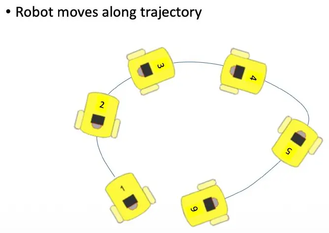
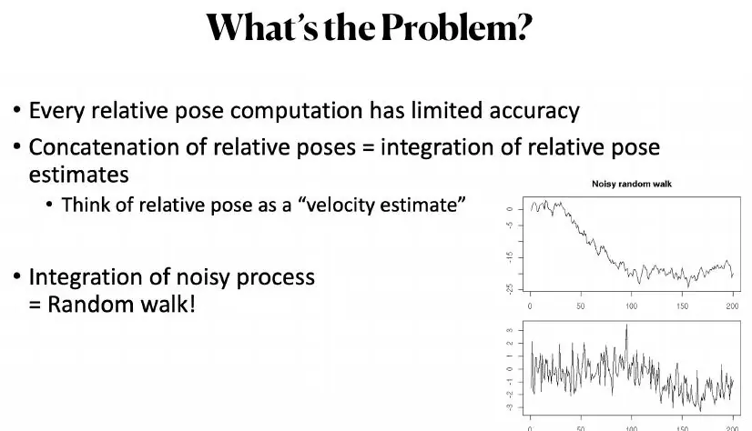
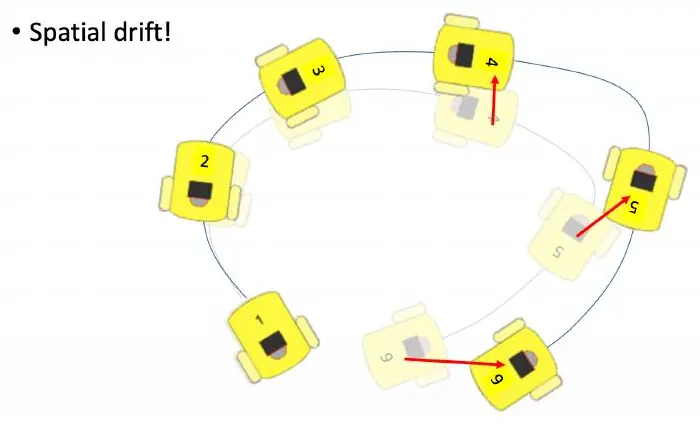
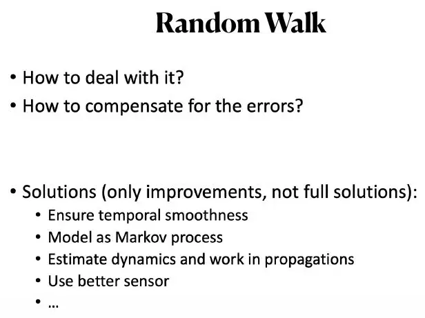
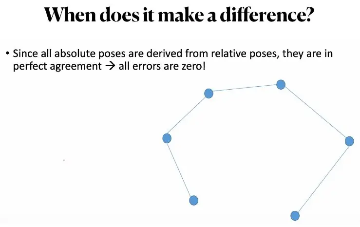
The reference-analysis lecture studies a robot moving around a loop. Integrating noisy relative motion creates random-walk drift: every local error is carried into later poses, so the final pose fails to meet the start. The remedy is not arbitrary smoothing; it is to represent all relative measurements as graph constraints and optimize the absolute poses jointly.

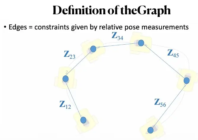
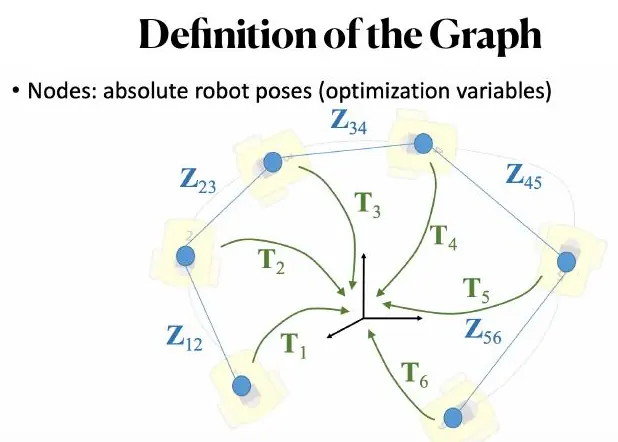
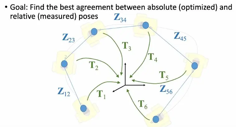
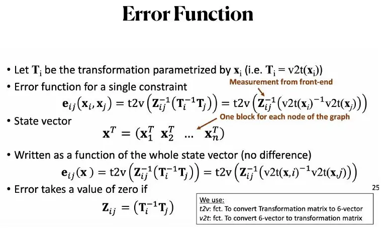
Let node pose be transformationand edge measurementfromto. A local error can be written in the tangent space of the transformation group:

With information matrix, solve

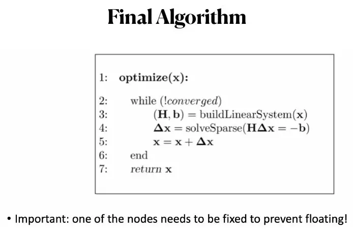
One pose must be fixed to remove gauge freedom: relative measurements cannot determine the global origin. Robust loss may downweight false loop closures, but should be justified by residual diagnostics.

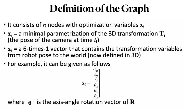
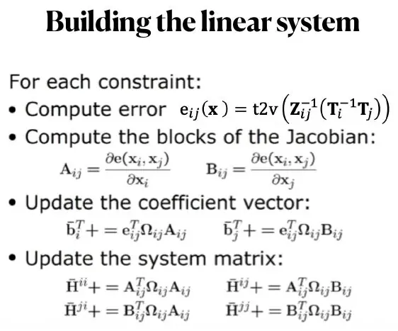
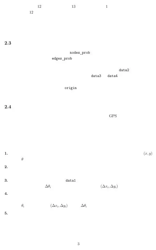
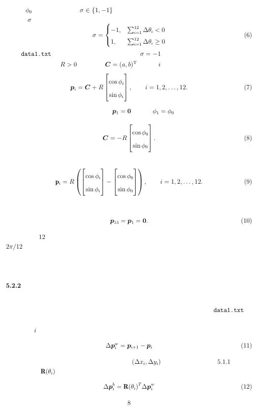
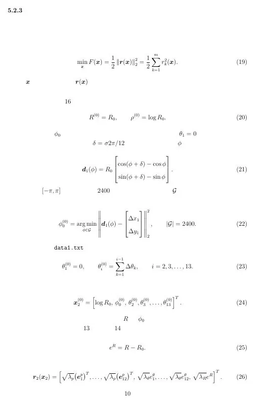
The first graph images above give us a reading sequence rather than a collection of answers. The early loop drawings show how local increments accumulate into a global gap. The later node-and-edge drawings show the change in representation: we no longer treat the plotted path as a sequence to be cosmetically smoothed; we treat measured relations as constraints that can disagree. The pose parameterization figure matters because coordinates used for a numerical update are not automatically the same object as a rigid transformation composed between frames.

Before trusting a pose-graph formula in a lecture or paper, trace one edge. If a measurementmaps poseto pose, compare it with the model’s predicted relative transformin the same direction and coordinate convention. Reversing the measurement without inverting it can yield a plausible-looking but wrong loop. A three-node hand example is ideal for this check because you can write each displacement and transformation explicitly.

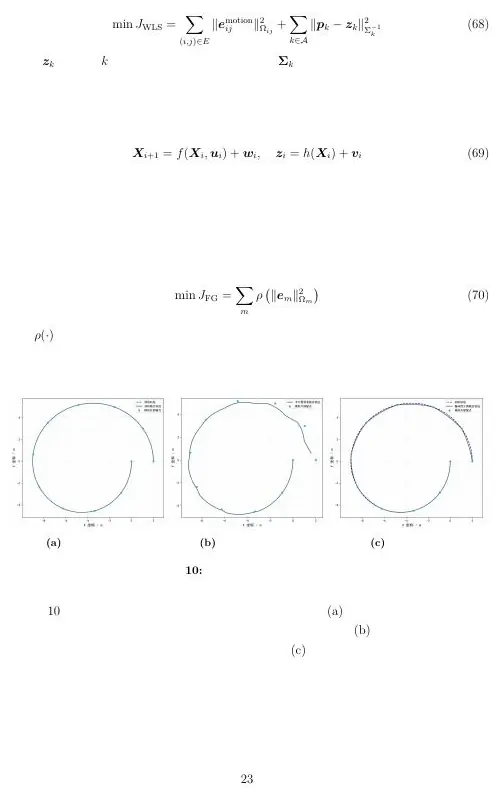
The residual pictures later on the page should then be read as diagnostics. A short residual arrow on every edge is evidence that constraints agree under the model and assigned confidence. One very large arrow is not fixed by reporting a small average over hundreds of edges. Ask whether it is a real outlier, a false loop match, a coordinate-frame error, or a covariance that was underestimated. The picture belongs at the point where we explain that diagnostic, not in an appendix as visual decoration.

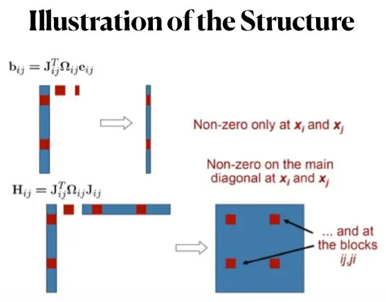
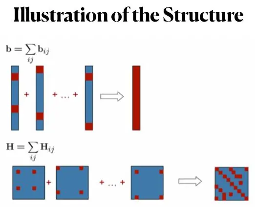
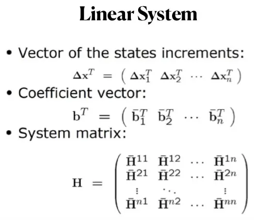
Finally, the sparse-matrix figures are the computational consequence of the node-edge graph. They are not new assumptions about the robot. Each edge contributes to a few blocks, so the algorithm can assemble and solve the system without allocating a full dense matrix for unrelated node pairs. In a competition paper, a small image of this block structure can justify a computational design choice more clearly than a paragraph claiming that the implementation is “efficient.”

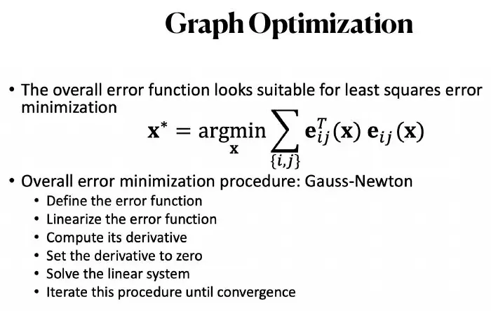
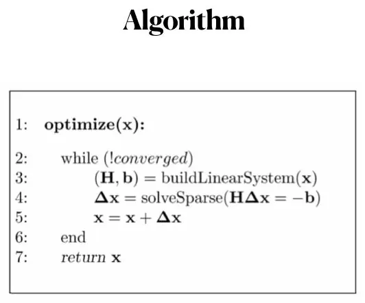
Gauss–Newton linearizesand solves

Because each edge touches only two nodes,,, and the linear system are sparse. Exploiting sparsity changes a seemingly huge problem into a practical one.

Competition preparation shown in the course

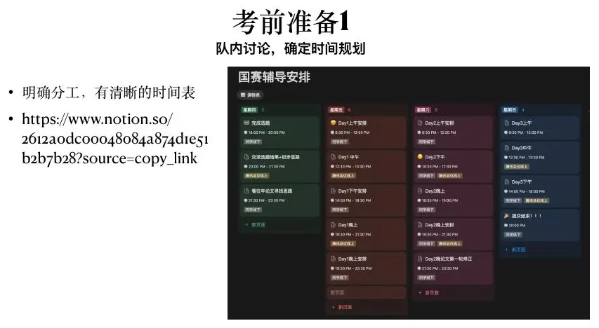
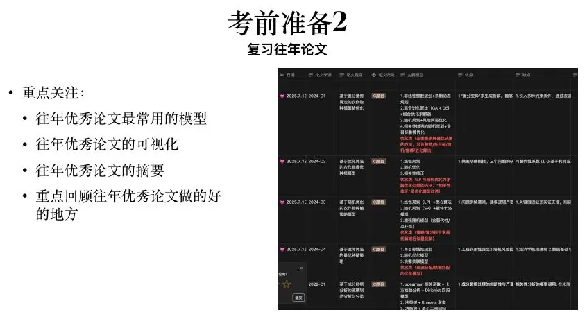
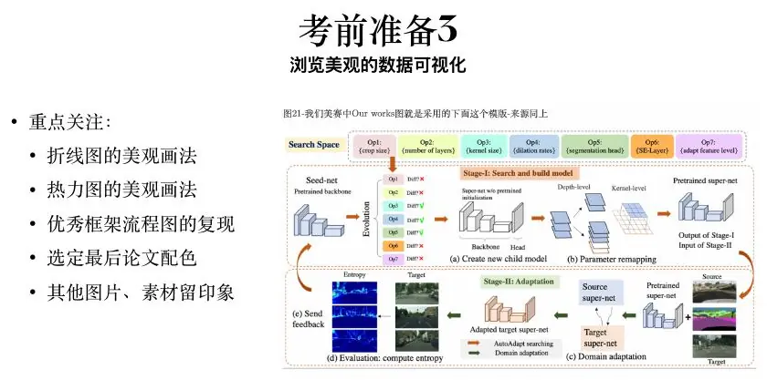
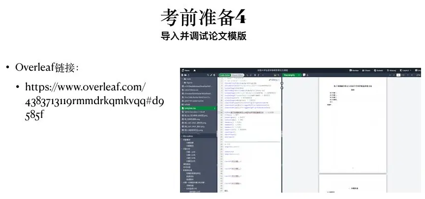
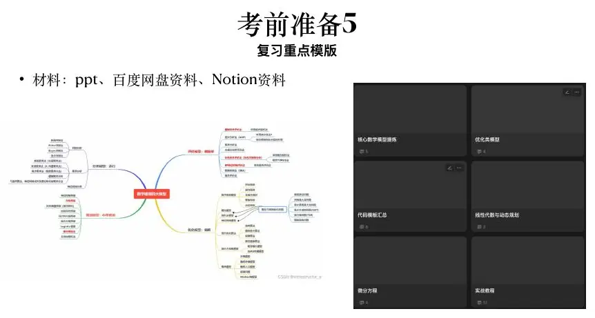
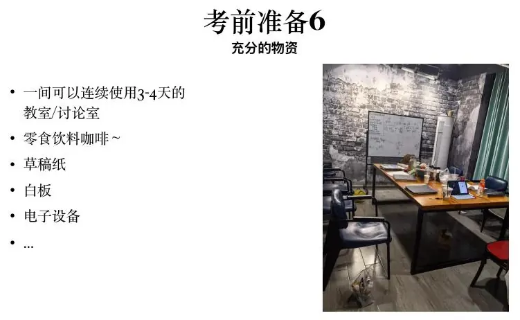
The final lecture covers logistics as part of modeling quality: install and test the environment, prepare templates, collect trustworthy references, agree on file ownership, practice diagrams, and make an offline fallback. During competition, inspect all prompts before choosing; check data accessibility, team fit, model opportunities, and the risk of an attractive but underspecified problem.

Second mock case: read figures as a model pipeline

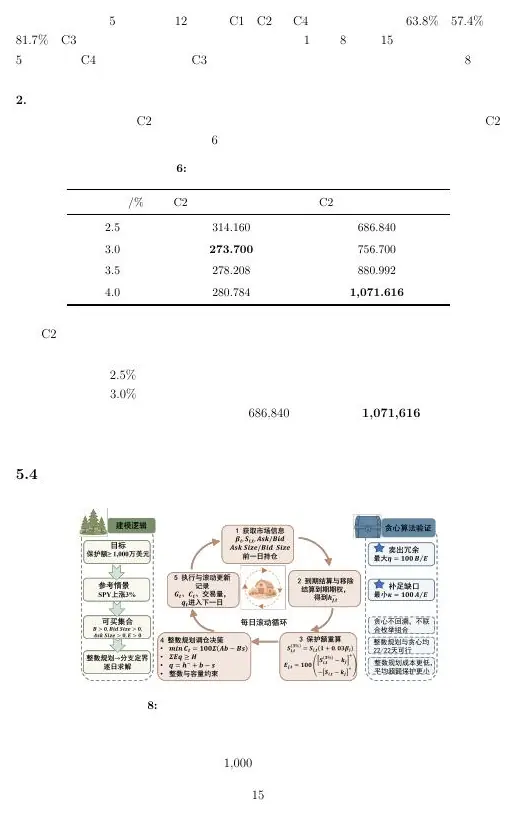
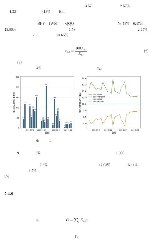
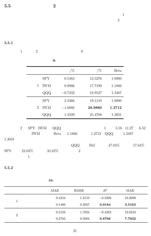
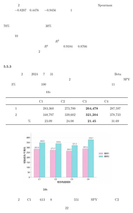
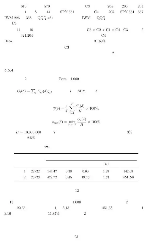
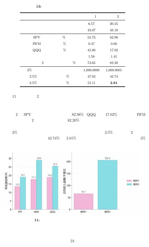
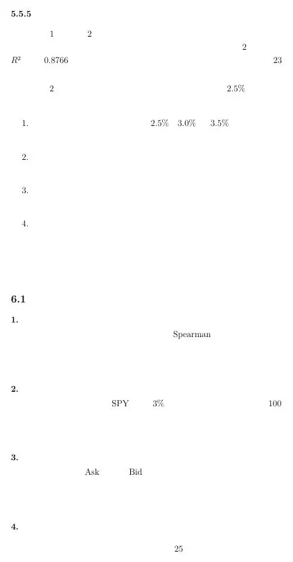
The second mock material contains process architecture, time-series comparisons, heat maps, regression diagnostics, and final strategy comparisons. Use them as a cold-reading exercise: reconstruct the question, variables, method, result, and limitation from each figure, then check whether the caption supports that reconstruction.

A figure is a bridge between modules

Consider the time-series panel in the gallery below. It may contain several curves, but a useful interpretation begins with axes: what quantity is on the vertical axis, in what unit, over what dates, and which curve is observed rather than predicted? If the forecast line is plotted over training dates only, it may show fit, not predictive performance. If a shaded band is present, ask whether it is a confidence interval for a mean, a prediction interval for future observations, or simply a range of scenarios. The picture cannot answer those questions without a precise caption and methods reference.

Now look at a heat map. The colors may show correlations, transition probabilities, risk levels, or policy interactions. A red square has no transferable meaning until the axes and scale are defined. If it depicts pairwise correlations between district risks, it can motivate a shared climate scenario rather than independent shocks. If it depicts an intervention coverage matrix, it can show which projects benefit the same residents and where additivity would double-count. The same visual form serves different mathematical claims. The figure should tell the reader which one is intended.

Regression panels often compare observed points with a fitted curve. A close line does not establish causality, and a high in-sample fit may be misleading if the policy uses the model in another year or district. Show residual patterns and held-out behavior when the claim is prediction. If the claim is explanation, identify possible confounders and the assumptions needed to interpret a coefficient. A graph is evidence only when its design matches the claim.

The final strategy bars should show feasible alternatives under a common budget and scenario set. If one strategy receives 6 million and another 8 million, the taller benefit bar is not a fair comparison. If one includes operating cost and another only construction cost, the cost bars are inconsistent. If uncertainty ranges overlap, a precise first-place label may overstate the result. The gallery’s visual sequence—from architecture to measurements, fit, sensitivity, and final options—is useful precisely because it invites these questions.

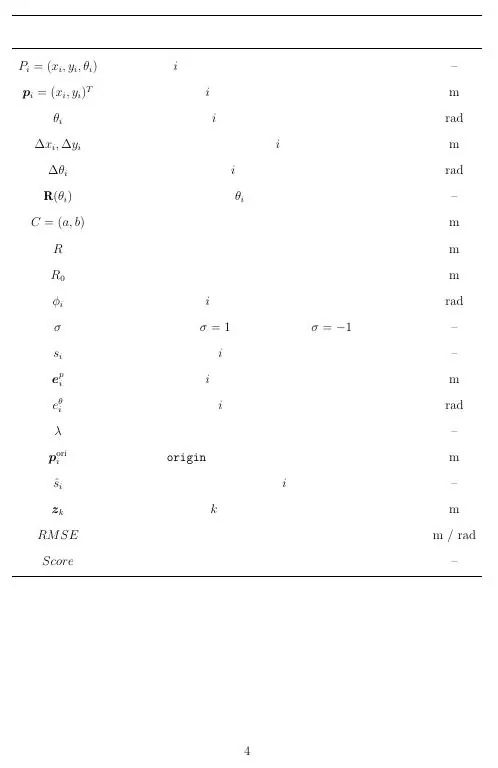
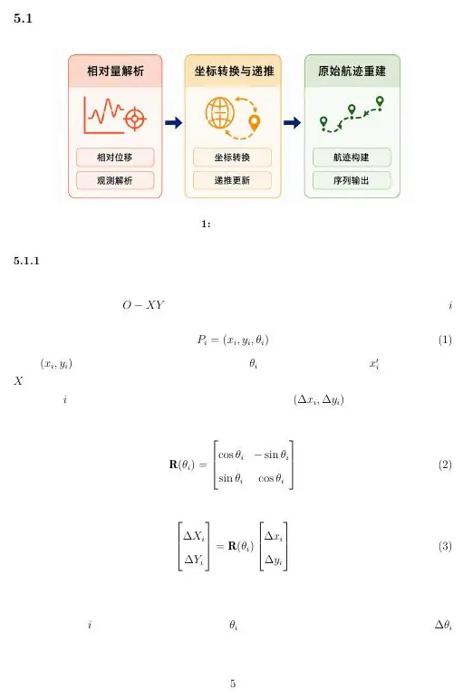
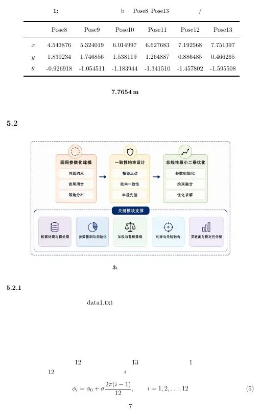
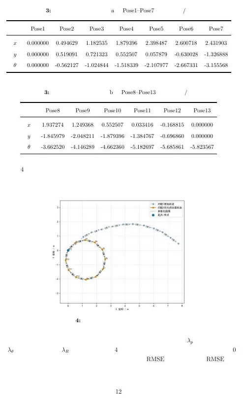
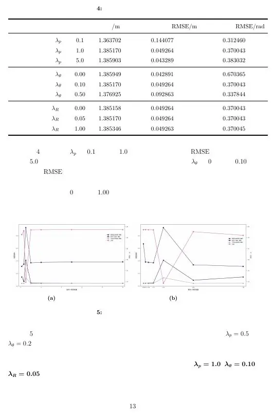
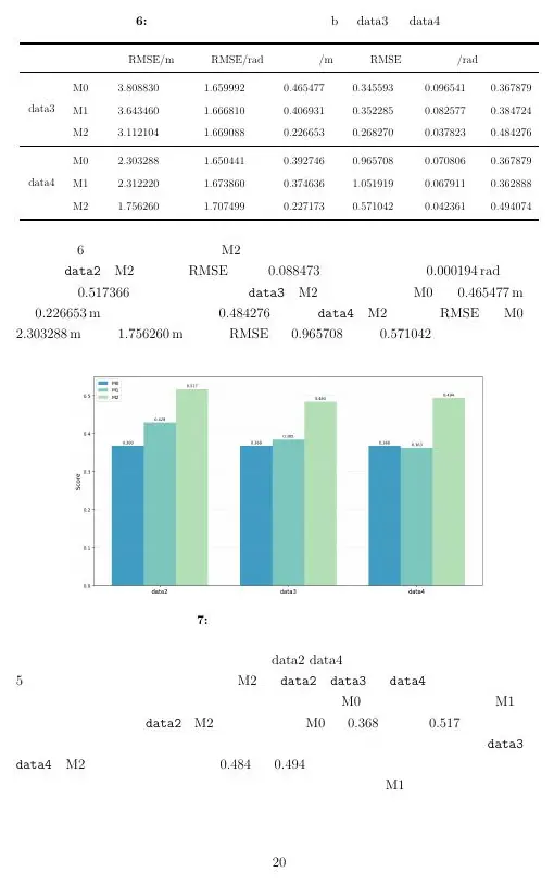
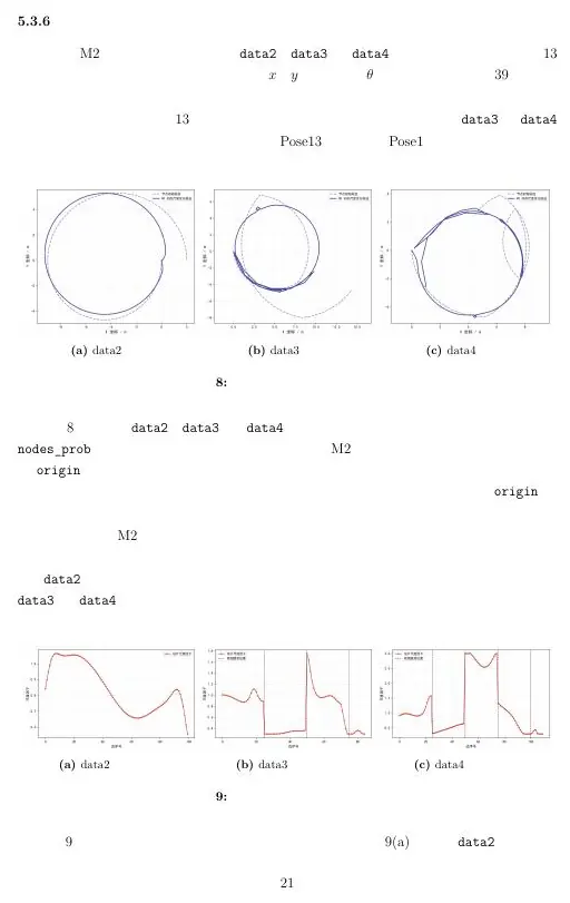
The first mock-submission figures later on the page offer another chance to see the chain. A process diagram should identify actual transformations between data and modules. A geometric output should preserve scale and units. A ranking table should include criteria, weights, and raw measurements or at least a path back to them. No figure has to be spectacular; it has to let a reader connect the prompt to a decision without filling in missing reasoning from their imagination.

When the paper is drafted, move a figure to the paragraph that needs it, not to a giant end-of-paper gallery. The related text should state what the figure shows, what claim it supports, and what it cannot establish. That habit keeps both the scientific argument and the reading experience coherent. It also catches orphaned graphics: if no sentence needs a picture, perhaps the picture does not belong in the main report.

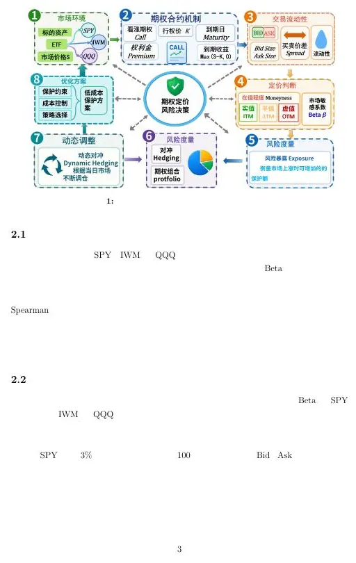
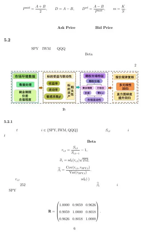
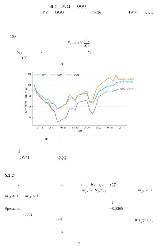
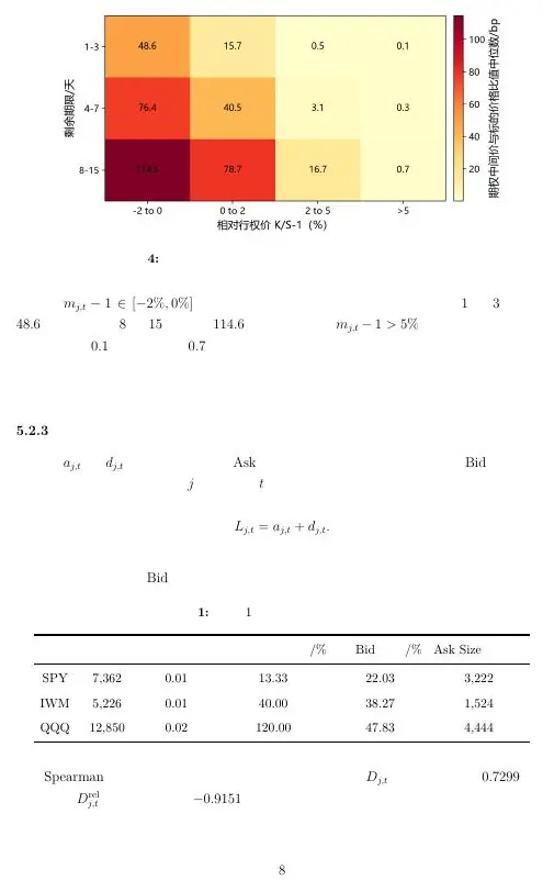
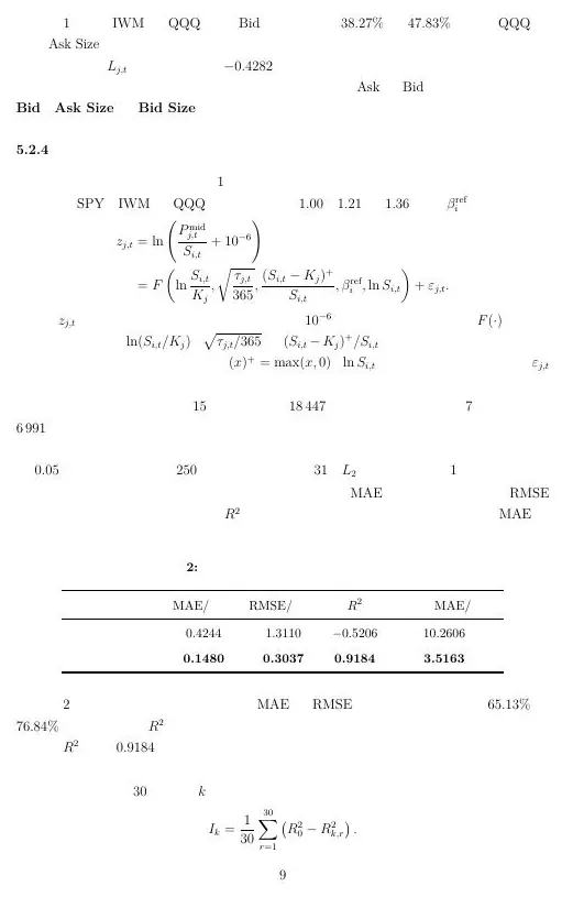
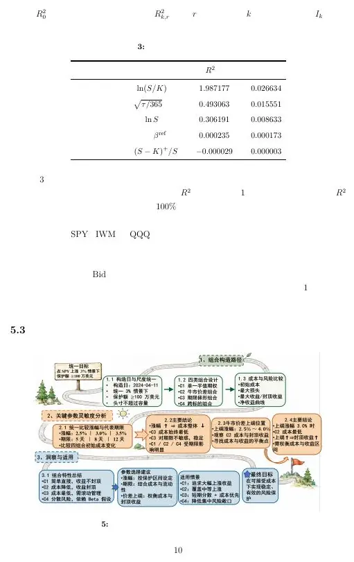
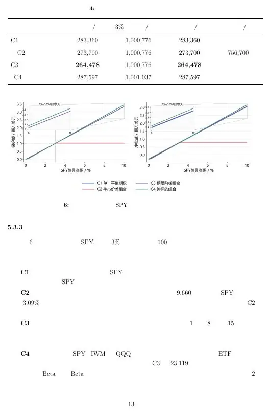
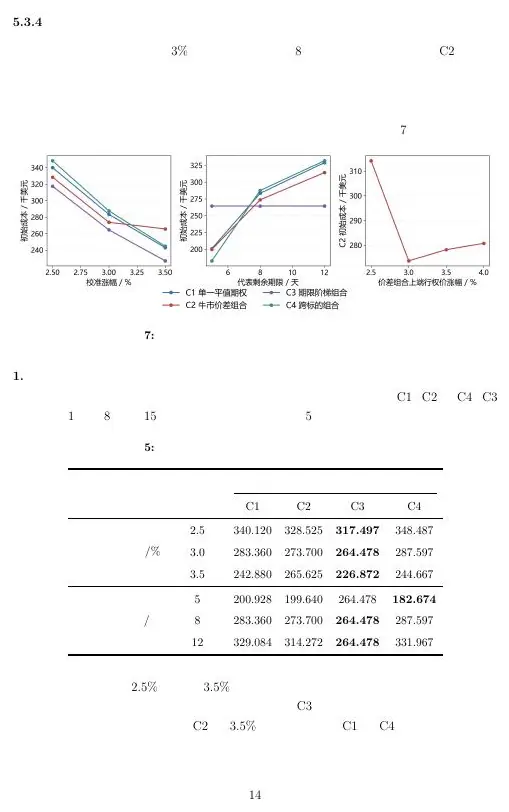
We have seen the model modules and the report structure. The following competition rehearsal joins them under a realistic deadline: the team must settle a question, test a baseline, and stop polishing before the files freeze.

A complete mock competition, from question to decision

Let us rehearse the opening of a competition. The prompt gives a large table of noisy measurements, asks us to explain the system, predict future behavior, and recommend a policy. The team’s first temptation is to split the questions among three people and start coding. Resist until you have one shared interpretation of the outputs and their dependencies.

Build one shared interpretation

Every teammate reads the entire prompt and writes the requested outputs as concrete nouns: a cleaned dataset, an estimated state, a forecast, a decision policy, a sensitivity result. Compare interpretations line by line. Highlight ambiguous words such as “optimal,” “stable,” “important,” and “accurate.” These words do not yet define mathematical criteria.

Create a data dictionary immediately. For every column record unit, observational unit, time stamp meaning, valid range, missing-value code, and whether the value would be known when a future decision is made. Make a row-count ledger after every merge or filter. Losing 30% of the observations silently is not preprocessing; it is an undocumented change to the population.

Before building separate modules, write a provisional answer to every subproblem in one sentence. The answers may be crude, but they reveal whether the planned modules form a complete chain.

Establish the minimum complete pipeline

Build the least sophisticated method that produces every requested output. For noisy graph measurements, this may be anchored least squares. For forecasting, use persistence and seasonal naïve. For a decision problem, construct a feasible heuristic. For evaluation, begin with transparent normalization and equal weights.

Run the full pipeline on a small slice and save the outputs. Check coordinate frames, time order, units, and feasibility by hand. A baseline generated in the first three hours becomes a safety net: every later extension can be compared against it, and the team can still submit a coherent result if an ambitious method fails.

Write the methods skeleton while the baseline is being built. Each subsection should already contain the question, inputs, output, core equation or procedure, and planned validation. Blank spaces expose missing reasoning early enough to fix it.

Diagnose before extending

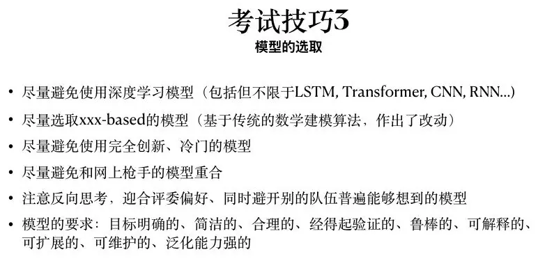
Do not add a neural network, metaheuristic, or complicated weighting scheme merely because it is familiar. Inspect where the baseline fails. Plot residuals against time, scale, geography, and operating regime. Check constraint violations and cases with large regret. Compare training and held-out error. The failure pattern chooses the extension.

If residual variance grows with magnitude, consider a transformation or heteroscedastic model. If a route heuristic violates capacity, improve the representation or repair rule before tuning search parameters. If a ranking changes under tiny weight perturbations, report instability and revisit the indicator system. Each extension should have a named failure mode and a planned ablation.

Maintain a model ledger with columns for version, hypothesis, change, validation design, result, decision, and owner. This prevents the team from remembering only the best-looking run and gives the paper an honest record of why the final model exists.

Create evidence, not screenshots

Freeze the evaluation protocol before extensive tuning. Use the same splits, scenarios, budgets, and metrics for every competing method. Run repeated seeds where randomness matters. Save raw metrics in a table from which all summary figures are generated.

Every important claim needs an evidence object. “The alignment is accurate” needs held-out residuals or an external reference. “The algorithm is robust” needs perturbation or scenario results. “The policy is better” needs a baseline under identical constraints. Assign each claim a table, figure, theorem, or diagnostic and put the reference into the draft immediately.

For the pose-graph case, check gauge freedom before trusting the optimizer. Fix one pose or add a justified prior. Verify relative-transform direction and rotation conventions on a three-node graph whose solution can be computed manually. Then inspect residuals by edge type; a low global cost can still hide a few destructive loop closures.

Integrate uncertainty and interpretation

Separate parameter uncertainty, data noise, scenario uncertainty, and model-form uncertainty. Not all of them need the same machinery. Bootstrap intervals can describe sampling variation; Monte Carlo scenarios can propagate uncertain inputs; alternative model families can expose structural dependence; robust optimization can protect a decision against a declared uncertainty set.

Translate uncertainty into the decision. If several parameter values produce the same facility locations, the recommendation is stable even if the precise objective varies. If a small plausible change reverses the chosen policy, the honest conclusion is conditional. A sensitivity result is useful when it tells the decision maker what must be measured or monitored next.

Write limitations as boundaries, not apologies. “The model assumes demand scenarios preserve the observed spatial correlation; independent site shocks were not evaluated” is precise and actionable. “Due to limited time, the model may have errors” tells the reader nothing.

Make the paper reproducible

Rerun the analysis from a clean directory. The program should recreate every table and figure from declared inputs. Store random seeds and software versions. Remove manual numbers from prose by generating a result table or at least maintaining a traceability sheet that maps each reported value to an output file and code location.

Audit notation across sections. A symbol must not change meaning between estimation and optimization. Check that every index range is declared, every equation is dimensionally consistent, and every constraint can be read as a real rule. Captions should state the comparison, metric, direction of improvement, and main conclusion.

Ask one teammate who did not write a section to reproduce its central claim. Cross-review is more effective than self-review because authors automatically fill gaps with knowledge that never reached the page.

Freeze and verify

Stop changing the model. Regenerate the PDF, inspect every page, confirm fonts and equations, and check that figures remain readable at actual size. Search for placeholders, stale references, unexplained acronyms, and contradictory numbers. Recalculate a sample of totals and metrics independently.

Read the abstract next to the conclusion. They should report the same methods and numbers at different levels of detail. Read every recommendation next to its assumptions and sensitivity range. Confirm that the title and keywords describe what the paper actually contributes.

The final question is simple: can a skeptical reader trace the path from prompt to data, from data to model, from model to evidence, and from evidence to recommendation? If the answer is yes, the work is competition-ready. If the answer is no, another algorithm will not save it; repair the chain.

Instructor’s debrief

A strong competition paper usually has fewer ideas than a weak one, but each idea is carried farther. The baseline is explicit. The main extension answers an observed failure. Validation mirrors the deployment situation. Sensitivity changes the interpretation. Figures carry claims. The recommendation is bounded by assumptions.

When you practice, score yourself on completeness before sophistication. Could another team reproduce the result? Can you explain one failed approach and what it taught you? Does each subproblem contribute to the final decision? Can you identify the single assumption most likely to reverse the conclusion? These questions reward modeling maturity rather than algorithm collecting.

The two mock problems are useful because they expose different weak points. A graph solution must explain frame conventions, the fixed reference, and residuals; a market solution must explain information timing and executable prices. If the written paper cannot explain its central question, validation, limitation, and recommendation without leaning on a software name, that is where the reasoning needs more work.

A final team rehearsal

Before the real competition, run one deliberately imperfect rehearsal. Give the team a prompt, a small dataset, and four hours. For the first thirty minutes, nobody is allowed to code. The team must produce the decision sentence, data dictionary, dependency graph, baseline, and validation plan. This constraint feels slow, but it usually saves time by preventing three people from implementing incompatible interpretations.

At the halfway point, stop and conduct a red-team review. One teammate argues that the data are insufficient, one tries to violate the model’s assumptions, and one attempts to reproduce a central number without help. Record every failure. Do not defend the work verbally; improve the artifact so that the answer becomes visible in code, equations, tables, or captions.

In the final hour, change one important input and one modeling assumption. A robust workflow should regenerate the affected outputs without manual repair. Ask which conclusions survive, which weaken, and which reverse. This rehearsal tests far more than programming: it tests whether the model is modular, the evidence is traceable, and the writing tells the same story as the computation.

After a rehearsal, each teammate can identify one decision that saved work, one interface that caused confusion, and one check that caught a real error. Convert those observations into a better team process. The purpose of practice is not to predict the next prompt; it is to stay reliable when the prompt is unfamiliar.

There is one more useful role in this rehearsal: the “curious judge.” This person is not trying to catch formatting mistakes. They repeatedly ask, “Why does this equation represent the situation?”, “How do you know this improvement is real?”, and “What would make you change the recommendation?” A team that can answer those questions with evidence has probably built a coherent model. A team that answers with software names has probably skipped part of the reasoning chain.

After the rehearsal, keep the artifacts that are reusable: plotting functions, table styles, solver-audit code, time-aware validation utilities, unit checks, and the paper skeleton. Do not keep a giant black-box template that forces every future problem into the same method. The reusable asset is a disciplined workflow. On competition day, that workflow gives you enough calm to understand the new problem before trying to impress anyone with the solution.

Finally, remember that clarity is not a reduction in mathematical depth. The strongest paper can state a difficult idea in ordinary language, express it precisely in mathematics, verify it computationally, and return to ordinary language with a bounded recommendation. That four-step movement is what the studio is training.

Close the heat case without pretending it is certain

Let us imagine the final heat-project presentation to a city committee. We do not start with the optimizer name. We say that the current district data suggest North and South carry the largest modeled exposure, and that under a 6-million budget the three-project baseline selects North’s center expansion and South’s retrofit. Those two projects cost 2 and 4 million, and their assumed avoided exposure adds to 8,000 risky person-days. The reader has already seen where those numbers came from and what they do not measure.

The committee asks, “Why not fund Central too?” We should not answer, “Because the solver did not choose it.” Central’s shade project costs 1 million, so adding it to North plus South would raise total cost to 7 million and violate the stated cap. The alternative Central plus South costs 5 million but has a nominal benefit of 6,000 under our coefficients. If there is an independent cooling-access requirement for Central, then the original plan may be unlawful or ineffective, and the optimization must include that requirement. This explanation makes the budget and service rule visible as reasons, not as opaque software behavior.

The committee asks, “Are 8,000 people kept safe?” No. The unit is modeled person-days of risky heat exposure avoided, not distinct people and not medical outcomes. The estimate assumes a specific efficacy for each intervention and a district-level exposure proxy. We should say so plainly. A single resident could contribute several days to the count. A benefit realized over several summers cannot be assigned entirely to next summer. Precision in terminology prevents the paper’s calculation from turning into a public promise it never supported.

The committee asks, “What if next summer is much hotter?” We can rerun the plan under high-heat scenarios, but first specify what changes: forecast dangerous days, project efficacy, operating capacity, or all of them. If North’s center has a maximum daily capacity, hotter weather may make its benefit saturate. If the South retrofit affects a fixed set of buildings, its avoided exposure may rise with heat until some physical limit. A robust recommendation describes which mechanisms were perturbed, rather than simply announcing that 10,000 simulations were performed.

Suppose that in a plausible low-efficacy scenario South’s retrofit avoids only 3,500 risky person-days. North plus South then yields 6,500 under additivity, still larger than the nominal Central plus South total of 4,500 and the North plus Central total of 4,000. But this comparison uses Central and North benefits held fixed; if those benefits also change with temperature, we must compare all plans under the same scenario. A fair scenario table has one row per shared set of assumptions and one column per feasible portfolio. Selecting a plan from one scenario and evaluating a competitor in another would be a hidden comparison error.

Suppose another scenario raises South’s retrofit cost to 4.5 million. North plus South now costs 6.5, so it fails the 6-million cap regardless of how attractive its benefit remains. Central plus South costs 5.5 and may become the feasible high-benefit alternative. This is a threshold transition, not a smooth small change in score. A cost range that crosses a budget constraint should receive prominent attention in the conclusion and may justify seeking a firm construction quote before committing.

These are not hypothetical details added to decorate a recommendation. They are exactly the conditions under which the city would make a different choice. The baseline taught us the nominal answer; sensitivity identifies the fragile inputs and binding rules; validation tells us which computations and measurements have been checked. Writing then turns those findings into a bounded proposal that a person can use.

We can also explain why no advanced forecast, AHP hierarchy, or network optimizer appears in the final recommendation unless it earned a role. Maybe a seasonal baseline predicts dangerous days well enough for this budget choice; maybe the available vulnerability indicators are too sparse for a responsible AHP score; maybe interventions in different districts do not overlap enough for network complexity to change the plan. Rejecting unnecessary methods is not a lack of ambition. It is evidence that the team understands which assumptions matter for the decision.

If richer evidence later arrives, the framework is ready to change. A new age-distribution table could refine vulnerability, an updated station map could refine exposure, a validated retrofit study could revise benefit coefficients, and an accessibility policy could add a hard constraint. Each update enters a named module and produces a traceable new recommendation. That is why a complete small baseline is so valuable: it gives the project a coherent structure that survives revision.

The studio closes where our first modeling lesson began: with a real question before a formula. A good competition paper makes the reader feel guided through the question, the evidence, the model, the checks, and the action. It does not ask the reader to admire a list of software packages or to trust a single rank without its conditions. If a skeptical teammate can reproduce the core calculation and explain when the recommendation would change, the team has produced more than a polished PDF. It has produced a usable piece of modeling reasoning.

First mock submission: evidence audit

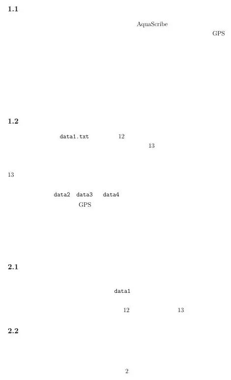
The first mock submission adds a second set of worked outputs. Rather than copying its formulas, use the images below to practice traceability: every architecture, fit, heat map, table, and robustness plot must map to a requirement, equation, and decision statement.