Mathematical Modeling 5 - Results and Validation

Our robot pipeline from the previous lesson could produce a remarkably smooth route and still be wrong: perhaps the sensor clocks were misaligned, or a scheduling rule was broken downstream. What test would catch the mistake before we recommend an action? Keep that question beside you as we distinguish checking the code from checking the model against the world.

We will build a small validation experiment, then return to robot fusion and scheduling. Every result will need its own level of evidence: an implementation check, a physical or logical sanity check, a comparison with withheld observations, and a stress test that matters to the decision. This is not extra ceremony after the “real” modeling. It is how a calculation earns the right to appear in a recommendation.

A solver returning success=True proves only that the solver stopped under its criteria. It does not prove that the model represents reality, the data pipeline is correct, or the recommendation is stable.

I would tell a new modeler to think of four nested questions. Did we compute what we wrote? That is verification. Did the written mechanism reproduce observations it was not tuned to flatter? That is empirical validation. Did the method beat a simpler alternative under the same conditions? That is comparison. Would the recommended action survive plausible errors and matter to the person who must act? That is decision validation. Passing the outer question requires attention to the inner ones, but passing an inner question alone does not answer the outer one.

In our robot case, a correct matrix implementation is a strong start; it does not certify that the constant-acceleration approximation handles every turn. A small RMSE on a path reference is useful; it does not certify every target-range window near a five-metre boundary. A solver certificate for selected candidates is useful; it does not certify that the candidate generator found every physically possible task. These are not reasons to abandon modeling. They tell us exactly what each result earns and which additional observation would let us recommend a plan more confidently.

In our bicycle case, conserving all fourteen bikes in the two-station toy is an implementation check. Beating a seasonal-naive forecast on withheld dates is a prediction check. Reducing unserved trips against do-nothing on matched days is a policy comparison. Keeping service acceptable on event days and under truck failure is a decision stress check. If any one fails, do not hide it by averaging with three green checks. Name the failure, its scope, and what action or model change follows.

When you read a result, ask which of those four questions it actually answers. “RMSE = 0.6301 m” is a path-error statement under an evaluation reference; it does not by itself answer whether a task window is safe. “27 tasks scheduled” is a decision-model output; it does not by itself answer whether sensor clocks were correctly synchronized. “MAE decreased” is a forecast statement; it does not by itself answer whether the overnight bike move improved service. The next figure or test should arise naturally from the unanswered question, which is how we keep a long article—and a real modeling project—from jumping between disconnected chapters.

I want you to leave this lesson with one sentence you can say in any team meeting: “What claim are we trying to support, and what observation could prove it wrong?” If a teammate answers only with a solver status or a beautiful chart, ask for the decision and the relevant baseline. That small conversation is the beginning of a credible results section.

Report results at three levels

Separate outputs into:

1. mathematical: parameter estimates, objective values, residuals, convergence;
2. domain: quantities with units, feasible schedules, predicted cases, ranked alternatives;
3. decision: what should be done, when, and under which conditions.

Every table and figure should be discussed. Do not repeat all values in prose; identify the dominant pattern, anomaly, or trade-off.

Let us translate the robot results through those three levels. At the mathematical level, the noisy attachment’s joint alignment estimates a-second clock offset and a spatial-bias vectormetres; its fused path has a reported RMSE ofmetres. At the domain level, we say the two positioning systems can be brought onto one 10-Hz path under the model’s timing and coordinate assumptions. At the decision level, that path can generate candidate windows for shooting and photography, yielding a schedule of 25 shooting and two photography tasks in the supplied report. A reader should not have to infer the task decision from a matrix of filter coefficients.

The field attachment has a different result. A candidate fixed bias of magnitudemetres improves RMS by onlyand makes BIC worse. The mathematical conclusion is that the extra fixed-bias parameters are not supported by that selected criterion and improvement scale. The domain conclusion is that a small residual mean in field data is not automatically a permanent sensor shift. The operational conclusion is to retain the no-fixed-bias field path for downstream task decisions, while monitoring for calibration drift. Reporting “we detected a bias” simply because a vector estimate was nonzero would reverse the meaning of the evidence.

Now imagine a table with a row for each attachment: noise-free, noisy with known fixed bias, and field measurements. Give each row its clock offset, whether a spatial correction was retained, position metric with units and evaluation set, output-point count when relevant, and main diagnostic. The table makes it harder to accidentally quote the idealized near-zero alignment error as if it belonged to the field case. In prose, do not recite every cell. Say what the table teaches: one easy attachment identifies the clock cleanly; noise and bias complicate fusion; field data can make a plausible correction unnecessary.

What would a decision-maker want to hear? “The selected schedule contains 27 modeled feasible tasks under the supplied resource and geometry rules, but target feasibility near distance or timing thresholds should be retested under position uncertainty.” That sentence does not claim every real-world attempt will succeed; it shows what the mathematical plan means and what remains to validate. An output is not a recommendation until its operating conditions are stated.

A results table is persuasive only after we know the calculation did what we wrote and the resulting claim survives comparison with observations. Keep these two questions separate: first check the implementation; then ask whether the model describes the world.

Verification before validation

Verification asks whether the implementation matches the intended mathematics. Use:

• unit tests on small known cases;
• independent recomputation of constraints and objective values;
• dimension and unit checks;
• conservation residuals;
• extreme cases where behavior is obvious;
• repeated runs for stochastic algorithms.

For an optimization solution, explicitly compute constraint violation:

$$
v=\max\left{\max_i(Ax^*-b)i,\ \max_j|A{eq}x^*-b_{eq}|_j,\ 0\right}.
$$

Feasibility tolerance should be stated, not assumed.

Let us practice verification before using the word “validated.” In the toy clock dataset, source 2’s printed times are three seconds ahead. If our alignment code outputswhen the report definesas an offset subtracted from source-2 time, either the code or the prose has the wrong sign. No real-world field test is needed to catch that implementation inconsistency. In the constant-speed filter toy,m/s overseconds should advancebym when acceleration is zero. A program that changesinstead has a state-order bug, however smooth its plotted trajectory looks.

For a task schedule, make three candidates by hand. Candidate A occupies 10:00–10:10 for the shooting device, B 10:05–10:15 for the same device, and C 10:06–10:08 for independent photography. The schedule may select A with C or B with C if both are individually feasible, but not A and B together. Ask a second script or teammate to recompute overlap from the exported selected-task table, not from internal solver flags. If it finds A and B together, the solution is not feasible under the intended rule even if the solver says success=True.

The displayed violation formula summarizes inequality and equality residuals, but be careful when constraints have different units. A capacity inequality may be in people, a time-window inequality in seconds, and a distance rule in metres. Taking a raw maximum across them is not a meaningful universal “small number.” Check each constraint group against a declared tolerance in its own unit, or scale residuals by an appropriate physical or numerical reference before comparing. A violation ofin a dimensionless binary logic check has a different meaning frommetres of distance orpeople. State the rule and tolerance that matter to the application.

Extreme cases are also verification tests. If all shooting candidates overlap, at most one can be selected for that device under a single-resource rule. If no task candidate passes the range limit, the selected count must be zero. If the clock overlap set is empty for a candidate shift, alignment should reject or penalize it rather than divide by zero or quietly return a tiny residual. If a model passes these simple cases, we know more about the implementation than we do from a giant result table whose correct answer is unknown.

Finally, perform conservation checks for stateful models. In the bicycle case below, moving bikes among stations should not change the citywide inventory. In the water basin from lesson one, energy lost by water should equal energy gained by a plate under the no-heater, no-room-loss assumption. In the coastal shelter example, residents assigned to shelters should sum to the demand, and shelter capacities should hold. Different domains have different invariants, but the habit is the same: identify what the code cannot create or destroy under the stated mechanism.

Validate against evidence

Choose tests appropriate to the task:

• regression: residual structure and out-of-sample error;
• forecasting: rolling-origin evaluation and prediction interval coverage;
• classification: confusion matrix and threshold-sensitive metrics;
• clustering: stability and domain interpretability;
• simulation: calibration and distributional comparison;
• optimization: baselines, bounds, and realized scenario performance.

Data leakage is especially dangerous. A scaler, feature selector, or imputer fitted using test data makes the evaluation optimistic.

Why is leakage a problem? Imagine the bike manager decides at 10:00 p.m. where to move bikes for tomorrow morning. She knows inventories tonight, past rentals, the calendar, and perhaps a weather forecast issued tonight. She does not know tomorrow’s actual rentals or the weather that will later be measured at noon. If your model uses those future values while reporting “next-day forecast accuracy,” it is not evaluating the manager’s decision. It is answering a much easier retrospective question.

Leakage can be less obvious. Suppose you normalize each station’s demand using the mean and maximum over the entire dataset, including the weeks you call “test.” The future’s scale has influenced the training features. Suppose you fill missing values with a median computed from all days, or choose predictor columns based on correlations calculated over all dates before splitting. Those operations expose test information to the model even if the final estimator never directly sees the test labels. Fit preprocessing on past training periods, then apply those learned transformations unchanged to later periods.

A random split is also risky for daily demand. If Monday of one week is in training and Tuesday of the same week is in testing, shared holiday or event patterns may make the test easier than a genuine future forecast. A rolling origin evaluates several realistic decision dates: train on information before date, predict days after, move the origin forward, and repeat. Each origin should recompute only what would have been known then. This shows whether performance is stable across seasons and special events rather than lucky on one randomly selected collection of rows.

For the repositioning policy, keep the decision time fixed in evaluation. On each withheld day, use the inventories and forecasts available at closing time, choose a move, and then replay actual or simulated next-day arrivals and returns. Do not allow the optimizer to “retune” its move after the true morning demand becomes known; that would be an oracle policy, useful as an upper bound perhaps, but not as an implementable recommendation. If you compare your policy with such an oracle, label it clearly.

The robot example has the same timeline issue. A backward-smoothed trajectory uses readings from later in the completed path. It can support an offline reconstruction and post-hoc schedule analysis, but it is not what an online robot knew before those later measurements existed. A results section should distinguish offline accuracy from real-time decision value. If the task is genuinely online, evaluate a filtered path using only readings up to each decision time. If the task uses a completed path to plan a later run, smoothing may be appropriate, but state that information setting.

Here is a beginner question that catches many leaks: “Could the person making this decision have known this number at the moment the decision was made?” Ask it for each feature, normalization parameter, calibration value, and tuning choice. If the answer is no, either remove the number from the policy’s information set or change the claim to retrospective analysis. A beautiful low error is not evidence of deployable performance when it borrows knowledge from the future.

Sensitivity is a decision map

One-at-a-time sensitivity varies parameterwhile holding others fixed. A normalized local measure is

For nonlinear or interacting models, use scenario grids, Monte Carlo sampling, or global methods. Report when the recommended decision changes, not only how an intermediate output changes.

Uncertainty analysis asks “what outputs follow from uncertain inputs?” Sensitivity analysis asks “which uncertain inputs matter most?” They answer different questions and are strongest together.

Let us slow down with the two-station bicycle choice. Under the teaching forecast, moving two bikes avoids both shortages. If station 2’s demand rises from two to four, the same move creates two shortages there. The input changed—station-2 demand—and the output of interest is not merely the optimizer’s cost; it is the recommended move and the number of unserved trips at each station. A sensitivity table might show demand at station 2 equal to 2, 3, and 4 and record whether the best move is two, one, or zero under the chosen cost rule. The point where the recommended move switches is especially important to the manager.

The normalized measurecompares percentage change in an output with percentage change in one input near a declared baseline. If a 10% demand increase produces a 20% shortage increase, a local sensitivity of roughly two describes that response. But be careful whenor: a percentage change relative to zero is undefined. In our no-shortage nominal bicycle plan, use absolute shortage change, a finite-difference slope in bikes per bike of demand, or the threshold at which shortage appears. Do not force a divide-by-zero percentage because the formula looks sophisticated.

One-at-a-time tests are helpful for diagnosis. Vary station-1 demand while holding station 2 fixed; then vary station-2 demand; then vary truck cost. You can see which input first reverses the move. But a rainy citywide event may raise demand at both stations together. Testing each in isolation can miss a joint failure. A scenario grid across both demands or coherent Monte Carlo scenarios reveals interactions. This is why a model report should distinguish a local sensitivity exercise from a full uncertainty propagation.

Now return to the robot. A-second change in clock offset might barely alter overall RMSE but shift a task’s preparation window across a distance threshold. The decision may change sharply even when a global average error changes smoothly. Plot task count and selected task IDs against offset, target-coordinate perturbations, range limit, and motion threshold—not only RMSE against those inputs. If a task disappears after a tiny perturbation, label it conditional and consider a safety margin. If 20 tasks remain selected across all tested calibrations, those form a more dependable core schedule.

Uncertainty propagation asks what happens when we draw plausible errors together. For each draw, shift calibration parameters according to their estimated joint uncertainty, reconstruct or perturb the path, regenerate task windows, and solve the schedule again. Record selection frequency for each task and distribution of final count. If you hold candidate windows fixed while varying only the final optimizer, you have not propagated uncertainty from sensors into decisions. The whole pipeline needs to be rerun along the arrows from lesson four.

Finally, do not call a recommendation robust simply because one sensitivity graph is flat. State the tested ranges, which parameters moved jointly, how those ranges were justified, and what failure boundary was found. A manager can use “this plan stays feasible for demand between 80 and 100 bikes per hour but fails above 105” far more readily than “the method exhibits good robustness.”

Compare models fairly

Use the same train/test split, objective definition, constraints, and evaluation metric. Include a simple baseline. A complex model that improves training fit but not held-out performance should not be presented as progress.

When multiple criteria matter, show the trade-off rather than hiding it in one weighted score. A Pareto frontier often communicates more than declaring one arbitrary weight vector optimal.

For the robot, imagine comparing source 1 alone, source 2 after alignment, a simple average of aligned readings, a filter, and an offline smoother. If the filter is evaluated on the easy noise-free attachment while the single-sensor baseline is evaluated on noisy field measurements, the “filter wins” sentence is meaningless. Put every method on the same time interval, coordinate frame, reference path, and position metric. State whether each method may use future observations. The smoother’s offline error should not be compared with a real-time filter as if they had identical information sets.

For bikes, compare repositioning strategies on the same withheld mornings. The do-nothing policy has zero truck distance and possibly more shortage. A simple heuristic may move bikes based on yesterday’s shortage. The proposed optimizer may lower unserved trips but spend more driving time. Make a table with both outcomes and a decision rule. If cost and service are both objectives, show several nondominated alternatives: perhaps plan A costsand leaves 20 trips unserved, plan B costsand leaves 12, and plan C costsand leaves 10. Whether the extrafrom B to C is worth two fewer failures is a value judgment, not something a plotting library can decide.

Training fit is not a fair result comparison. A complicated demand model can fit past station counts more closely than a seasonal rule and still forecast future event weeks worse. A bias-corrected robot path can reduce residuals on the same segment used to estimatebut worsen a withheld segment. An optimization model can lower its own objective by omitting a real device constraint. All three are forms of apparent improvement that vanish when evaluation matches the intended use.

Compare decisions, not only intermediate metrics. If a forecast reduces MAE from two bikes to one bike but never changes the recommended move, its operational value may be small for this policy. If a tiny clock calibration change swaps five robot tasks, the task decision is sensitive even though global RMSE barely moves. The results narrative should say which improvement mattered to the original question and which was only a mathematical refinement.

Write limitations precisely

Useful limitations identify a mechanism and consequence:

The demand model assumes the historical weekly cycle persists; a structural schedule change would bias the forecast and could make the staffing plan infeasible.

“The model is somewhat idealized” says nothing. Follow each important limitation with a monitoring rule, mitigation, or extension.

Take the bicycle policy. It assumes the past daily pattern is informative about tomorrow and that the overnight truck can finish its route before demand begins. A better limitation says: “If a campus event changes morning arrival patterns or a vehicle delay prevents the planned move, stations chosen near zero spare inventory may experience shortages. We would monitor reservation and rental peaks, maintain a fallback no-move or partial-move rule, and reforecast after event notices.” The statement names a mechanism, consequence, observation, and response. “Real life is complex” names none.

Take the robot alignment. The body assumes one fixed clock offset. A useful limitation says: “If relative clock drift changes during the recording, a singlecan align the middle of the path while shifting early and late task windows. We would compare offset estimates by time block and use an affine or piecewise clock map only if that pattern is repeatable.” That sentence tells us which diagnostic to watch and which model component to revise. It is much more useful than “sensor errors may exist.”

Take the fixed-bias decision. The report did not retain a field correction because its candidate magnitude, RMS improvement, and BIC did not justify two extra parameters. A careful limitation says that the decision is conditional on the available field record and selected diagnostics; later calibration data could reveal a stable bias. Monitor block-wise residual means or independent reference positions. Do not rewrite the result as “there is no bias under any circumstances.” A model-selection choice is not a physical proof of exactly zero.

Take the schedule. A 27-task count is based on generated candidate windows, selected state estimates, device rules, and target geometry. If a task sits just inside a range limit, position uncertainty may remove it. Report how many tasks remain feasible when position, clock offset, range, or preparation time are stressed. For a borderline task, a safety margin or manual review may be more responsible than using the nominal plan unchanged. The limitation should point to the choice it can affect, not just to a mathematical parameter.

Limitations are strongest when placed near the result they qualify. A figure showing bike shortage by day can caption the event-day failures; a trajectory plot can mark uncertain turn segments; a task-window plot can shade boundary-sensitive candidates. Do not hide all caveats in a final paragraph after several pages of unconditional praise. A reader may never connect “the clock might drift” at the end with “the task schedule is feasible” at the beginning unless the bridge is written explicitly.

The conclusion should not introduce a completely new model to repair every limitation. It should answer the original decision under the evidence actually gathered and identify a monitoring trigger. “Use the proposed overnight bike move on ordinary weekdays; switch to an event-day fallback when predicted demand at the transfer hub rises above the tested range” is actionable if that threshold was tested. If it was not, say what test remains before deployment. That is honest, not weak.

Reproducibility package

The final supporting material should include source code, a data dictionary, preprocessing rules, random seeds, environment information, and a one-command execution path. Keep exploratory notebooks, but extract the final pipeline so that outputs can be regenerated from raw data.

The conclusion should contain no new method. It should answer the original questions, state the strongest quantitative evidence, describe the valid operating range, and end with the decision—not with a generic claim that the model is useful.

What does a one-command execution path look like conceptually? A teammate should be able to start from the preserved raw files, run the declared cleaning and alignment steps, regenerate fitted parameters, produce trajectory or demand predictions, solve the decision model, and then reproduce the exact tables and figures used in the report. That does not mean hiding the entire process in one opaque script. It means there is one documented entry point that calls understandable stages in the correct order and records the data and software versions used.

For the robot case, the data dictionary should define every sensor timestamp, coordinate unit, source ID, and target location. A preprocessing note should state how missing records, interpolation, and common-grid resampling are handled. A calibration result file should hold, any retained, and their diagnostic metrics. The 10-Hz path file should say whether it is filtered online or backward-smoothed offline. The candidate-task file should include rejection reasons. The selected schedule should include exact intervals and resource assignments. If these artifacts have stable meanings, a reader can trace the reported 27 tasks backward without relying on the authors’ memory.

For the bicycle case, record station inventory snapshots, rentals and returns, event calendar, forecast issue time, and truck movement costs. Preserve the rolling-origin split dates and the parameters fitted at each origin. If a future dataset changes, rerun the whole pipeline rather than pasting a new number into an old bar chart. Keep random seeds for simulations so a surprising scenario can be reproduced; run several seeds for conclusions that depend on random variation so one seed does not become the evidence by itself.

Reproducibility includes privacy and scope. Do not upload private rider or sensor records into a public repository merely to make the code easy to run. A public report can provide a schema, synthetic example, permitted aggregate data, and scripts that run when authorized data are supplied. State what parts of an analysis are reproducible from public files and what parts require restricted data. “All results are reproducible” is another unsupported claim if the underlying observations are inaccessible or undisclosed.

Before final submission, give the pipeline to someone who did not build it. Ask them to recreate one headline number from the inputs. If they cannot find the correct data version, do not know whetheris positive or negative, or cannot tell which schedule file is final, the package is not yet clear enough. A reproducibility test is also an editorial test: the report’s methods, table labels, and code need to describe the same model.

Test the claims behind a result

Suppose a model predicts daily bicycle demand and an optimization model uses those predictions to reposition bicycles overnight. A low forecast error does not automatically imply a useful repositioning policy. Validation must follow the complete chain from prediction to decision.

Two stations before a citywide model

Imagine you manage a bike-share system with just two stations. At closing time, station 1 holds ten usable bikes and station 2 holds four. Tomorrow morning, your first rough forecast is twelve rentals at station 1 and two at station 2 before any returns. A truck can move bikes overnight from station 2 to station 1. How many should it move? Write a guess before we calculate. Moving every bike from station 2 would leave its own morning riders without one, so the word “reposition” already involves a trade-off.

If you move none, station 1 is short by two bikes and station 2 has two spare. If you move one, the inventories are eleven and three; station 1 is short by one and station 2 has one spare. If you move two, inventories are twelve and two; both forecast demands are exactly covered. If you move three, the inventories are thirteen and one; station 2 becomes short by one. In this tiny fixed-demand example, moving two avoids all forecast shortages. But we have not included trucking cost, uncertain demand, damaged bikes, or riders returning bikes during the morning. “Two” is a baseline decision under a short list of assumptions, not the answer for the whole city.

Check conservation aloud: starting inventory isbikes. After moving two, it is. Repositioning changes location, not the total count. If a code run says station 1 has twelve and station 2 still has four, it has created two bikes from nowhere. That is a verification failure. If some bikes go to repair or leave service, the balance needs an explicit loss term; do not hide a real process inside an unexplained discrepancy.

Now add cost. Suppose moving each bike costsand leaving one customer without a bike has an estimated service penalty of. Under fixed forecasts, moving two costsand avoids two shortages. Moving one costsand leaves one shortage penalty of, total; doing nothing costsin shortage penalty; moving three costsplus one shortage penalty of, total. Under these invented teaching values, two remains best. But if truck cost rose toper bike, moving two would costand doing nothing would cost; the recommendation might change. The abstract or results section must say which objective and cost assumptions produced the choice.

What if the forecast is wrong? Suppose station 2’s morning demand is actually four. Moving two would leave it short by two, while the do-nothing plan would serve all four there and leave only station 1 short by two. Total shortage is equal in that outcome, but service distribution and trucking cost differ. If demand at both stations rises together on sunny days, sampling their forecast errors independently could create unrealistic scenarios. We need a demand model that preserves citywide weather or event effects, or at least stress scenarios that vary both stations coherently.

This tiny case separates three things the report must not confuse: forecast accuracy, optimizer correctness under the forecast, and realized service under uncertain demand. An algorithm can solve the fixed-demand two-station objective exactly and still choose poorly on a sunny morning because the inputs were wrong. Conversely, a forecast with slightly higher citywide MAE might place more bikes at a critical station and improve service. The only way to decide is to evaluate the complete policy on future or realistic withheld days with the same information timeline as the overnight manager.

Establish three baselines

Use a seasonal-naive demand forecast, a do-nothing repositioning policy, and a simple rule that moves bicycles toward stations with yesterday’s shortage. The proposed pipeline must be compared with all three. This separates the contribution of forecasting from the contribution of optimization.

Evaluate on days not used to fit preprocessing, features, parameters, or hyperparameters. For temporal data, use rolling origins. Report MAE for demand, shortage trips for operations, and cost or driving distance for implementation. A forecast can improve MAE while worsening shortage if its errors occur at strategically important stations.

Let us make that last sentence concrete. Suppose a new demand model misses station 1 by ten bikes and gets nine quiet stations exactly right. An old model misses each of ten stations by two bikes. If we average absolute errors equally across stations, the new model’s MAE isbike and the old model’s isbikes. The new model “wins” on MAE. Yet if station 1 is the busy transfer hub where morning shortages cause many failed trips, its ten-bike miss may lead to far worse service than the old model’s distributed small errors. This is why forecast accuracy and policy value need separate metrics.

Measure demand error in bikes per station and time period. Measure service in unserved trip requests or a service-rate percentage with a stated denominator. Measure truck effort in kilometres, labour time, or dollars. These cannot be collapsed into one cheerful “model score” without a declared objective and weights. A manager may accept two more unserved trips to save an hour of overnight driving, or may forbid any shortage at a hospital-adjacent station. The report should show those trade-offs and constraints.

Pair policies on the same withheld day and scenario. Suppose the do-nothing rule yields 30 unserved trips on a rainy Monday and 5 on a sunny Tuesday, while the proposed rule yields 22 and 7. The proposed rule helps on Monday by eight but hurts on Tuesday by two. Their aggregate is 35 versus 29, a net six-trip reduction, but the day-level difference matters for deployment. Draw or tabulate paired daily differences, not just two unpaired means. If performance is concentrated in rain or large events, say so and consider a conditional policy.

Also report uncertainty honestly. If you simulated 1,000 days using one fitted demand distribution, a narrow Monte Carlo interval around the average shortage only tells you numerical precision under that distribution. It does not account for a wrong demand model or a future campus schedule change. Test alternate demand levels, correlated peak scenarios, and truck breakdowns. If the selected move changes under plausible inputs, the policy recommendation should be conditional or include a fallback rule.

Choose baselines with distinct jobs. A seasonal-naive forecast asks whether the new predictor adds useful information. A do-nothing policy asks whether moving bikes improves operations at all. A simple move-toward-yesterday’s-shortage rule asks whether the full optimization earns its complexity. Compare each using the same future days, available information, and cost rules. If the complex plan beats do-nothing but not the simple rule, the honest conclusion is that repositioning helps and the optimizer has not yet shown extra value.

Verify before validating

Construct a two-station problem that can be solved by hand. Check inventory conservation:

$$
I_{i,t+1}=I_{i,t}+\text{returns}{it}-\text{rentals}{it}
+\text{moved-in}{it}-\text{moved-out}{it}.
$$

Sum over stations. Internal repositioning should cancel. If total inventory changes without loss or repair, the implementation is wrong regardless of its attractive plots.

Propagate uncertainty with Monte Carlo simulation

Fit or justify distributions for demand residuals, travel time, and unavailable bicycles. For replication:

1. draw one coherent scenario;
2. run the fixed policy without retuning it using future information;
3. record shortage, operating cost, and service rate;
4. repeat with controlled random seeds.

Estimateand its Monte Carlo standard error. More simulations reduce numerical uncertainty in the estimate; they do not repair an incorrect scenario distribution. Plot the running mean and interval againstto justify the simulation budget.

Preserve correlation. Drawing station demands independently may eliminate city-wide peaks. Use residual blocks, copulas, multivariate models, or common scenario multipliers when dependence matters.

Let us make Monte Carlo less mystical. For one simulated morning, choose a coherent set of facts: rain or no rain, arrival counts at all stations, bike returns, travel time for the repositioning truck, and any bikes out of service. Feed the same morning to the current policy and proposed policy. Record unserved requests and trucking cost for both. Repeat for many mornings drawn or constructed by the stated scenario mechanism. Because each policy sees the same scenario, their difference is easier to interpret than two unrelated collections of random mornings.

Suppose five illustrative paired scenarios yield changes in unserved trips ofwhen moving from current to proposed policy. The average change istrips per scenario. Negative favors the proposed policy. But one scenario worsens by two trips, so we should inspect what made it different—perhaps station 2 demand spiked while the truck emptied it. With only five scenarios, we would not claim a stable expected reduction; the calculation is a hand exercise that shows what the simulation will summarize at larger scale.

Whenscenarios are simulated,estimates the mean outcome under the chosen scenario generator. The Monte Carlo standard errordescribes numerical variation in that estimated mean if scenarios are drawn independently under the model. If you quadruple, the standard error roughly halves. But if the generator underestimates rainy-day demand, running one million scenarios only estimates the wrong distribution more precisely. Validate the generator against observed frequency, joint peaks, and tail behavior before presenting a narrow interval as confidence in the real-world policy.

Correlation is a physical and behavioral issue, not just a statistical luxury. Rain might suppress rentals at many stations together; a city event might increase demand at several adjacent stations together; a transit outage might move demand toward bike stations near the affected line. Drawing each station independently can create unrealistic combinations and miss citywide pressure. A simple first repair is a shared scenario multiplier—on event days, raise demands together according to measured patterns. More advanced joint models can come later if data and decisions justify them.

Monte Carlo scenarios and deliberate stress cases have different jobs. The former help estimate how the policy performs across a declared uncertainty model. The latter ask how it fails at consequential boundaries: heavy rain plus truck breakdown, festival demand plus several damaged bikes, or two critical stations empty at once. The combined failure may be rare but costly. Report both ordinary distributional performance and a small number of named stress outcomes. “Works in 95% of simulated mornings” means little if the other 5% are precisely the days when a hospital district loses all bikes.

One practical test of simulation stability is a running-mean plot against the number of scenarios, with repeated batches using different seeds. If the estimate swings wildly even after thousands of runs, a rare high-cost outcome or poor scenario design may dominate. Inspect the tail rather than merely increasing. If it settles, you have reduced Monte Carlo noise, not necessarily calibrated the world. The distinction belongs in the results section whenever a simulation supports a decision.

Return to our five paired bicycle scenariosfor a moment. Their mean isunserved trips per scenario, but values range from an improvement of four to a worsening of two. A decision-maker cannot responsibly treatas a guaranteed saving every morning. With only five independent scenarios, the sample standard deviation is abouttrips and the Monte Carlo standard error of the mean is abouttrips. That numerical uncertainty is almost as large as the estimated average gain. We would need more well-designed scenarios before saying the average is stable, and we would still need to validate whether the scenario generator represents real mornings.

The paired differences also tell us what to investigate. Which scenario produced—the policy making service worse? If it was a station-2 event surge, consider a conditional move that keeps more bikes there when an event notice is available at decision time. If it was a truck delay, the issue may be operational rather than predictive. If it was a bad forecast on a quiet station, a better forecast metric might not solve it. A summary mean is a starting point for explanation, not the end of the results section.

Suppose we run 5,000 scenarios but 4,900 of them are ordinary weekdays and only 100 represent severe events. A policy could have a narrow-looking average improvement while failing the events that matter most to the manager. Do not “fix” this by arbitrarily giving events huge weights after seeing the result. Decide whether you are estimating ordinary expected service, evaluating an event-day policy, or checking a worst-case safety condition. Report the populations and weights separately so a reader knows what the mean describes.

For the robot schedule, the analogous summary is average task count under calibrated path perturbations. A mean of 26 tasks across scenarios can conceal a schedule that repeatedly loses the same critical photography task. Record task identity, not just count. If the mission values certain targets differently, a count objective may not match decision value. A validation report should make that mismatch visible and either explain the count-based scope or evaluate a declared reward metric.

These examples teach a simple habit: when you report an average, name the distribution over which you averaged, show one meaningful exception, and say whether that exception changes the action. When you report a confidence or simulation interval, name whether it describes uncertainty in the estimated mean, variation among future outcomes, or sensitivity to uncertain input parameters. An unlabeled shaded band cannot carry all three meanings at once.

Design stress tests, not only random tests

Random scenarios represent frequent uncertainty; stress scenarios examine consequential boundaries. Test a transit disruption, major event, heavy rain, and simultaneous vehicle failure. Report the threshold at which the recommendation changes. “The model works in 95% of sampled days” is incomplete unless the other 5% are understood.

Present a validation matrix

For each claim, list evidence and acceptance rule:

Claim	Evidence	Example acceptance rule
forecasts are useful	rolling holdout vs seasonal naive	lower MAE in at least 8 of 10 folds
solution is feasible	independent constraint audit	maximum violation
decision improves service	paired scenario comparison	lower shortage in at least 80% of scenarios
conclusion is stable	sensitivity and stress tests	selected policy unchanged over stated range

Define rules before examining the final results when possible. Otherwise it is easy to move the goalposts.

Imagine setting a success rule after seeing the proposed policy’s performance. If it reduces shortage on 79% of scenarios, we might suddenly declare “at least 75%” a success. If it reduces shortage on 81%, we might call “at least 80%” the original goal. The result looks the same mathematically, but the standard was chosen to flatter it. Set the acceptance rule from the decision-maker’s needs or a justified design target before the final test, and record changes with reasons. Exploration can still help us design a rule; it should not be presented as a predeclared independent test.

The matrix’s numerical toleranceis only an illustrative solver-scale value, not a universal physical requirement. A schedule’s binary overlap rule should be checked exactly on selected task intervals; a numerical distance limit should have a tolerance in metres appropriate to coordinate precision; a bike count should not permit 0.0000001 of a bike in an operational plan. For each claim, write the unit and what constitutes failure. This prevents one raw “constraint violation” number from blending incompatible dimensions.

For the robot, the validation plan might include: known-shift toy recovers the declared clock sign; segment-wise offsets agree within a stated tolerance under the constant-offset hypothesis; filter innovations do not show persistent turn-related structure; held-out path error is compared with aligned single-sensor baselines; field bias is retained only if improvement and complexity diagnostics support it; every selected task passes complete preparation-window, resource, and angle checks. These are different tests. A single smooth path overlay cannot stand in for all of them.

For the bike policy, the rows might include: future-period forecast beats a seasonal-naive baseline on declared MAE; inventory conservation holds exactly except for modeled loss or repair; shortage and trucking cost are compared against do-nothing and simple heuristics on matched withheld days; event and truck-failure scenarios are stress tested; and a policy-switch boundary is reported if the recommendation changes. Each row connects a claim to a dataset or toy case, a metric, a baseline, and a failure response.

Do not fill a matrix with only pass/fail ticks. Record the actual value or observed pattern beside each rule. “Passed rolling-origin evaluation” is less informative than “MAE lower than seasonal naive in eight of ten declared origins, but worse during two event weeks.” “Task schedule feasible” is less informative than “all selected intervals pass independently recomputed distance, speed, acceleration, overlap, and angle checks; two candidate tasks are within 0.2 m of the range boundary.” The exception often tells the team what to monitor next.

The matrix should also expose dependencies. If path reconstruction fails a calibration check, task-window validation based on that path is conditional even if the schedule code itself obeys overlap rules. In the report, distinguish “the optimization solved its modeled schedule correctly” from “the schedule is ready for a real robot.” The first is verification of one module. The second requires trustworthy upstream estimates and stress evidence. A connected results section lets the reader see that distinction.

Practice

Write one sentence that your model is intended to support. Decompose it into implementation, mechanism, empirical, comparative, and decision evidence. For each, specify a dataset or synthetic test, a metric, a baseline, and a failure threshold. This document becomes the validation plan and later the structure of the results section.

The first workshop established controlled comparisons. Let us now use the robot pipeline from the previous lesson: timing, spatial alignment, fused path, and task schedule must each be checked before a good final score can be trusted.

Validation continuation: robot fusion and scheduling

The robot case shows why a results section cannot be a parade of final numbers. Every module needs a diagnostic matched to its claim.

Start with the idealized attachment. It reports a-second offset and a maximum alignment discrepancy nearmetres. To verify implementation, use a known-offset toy path and check the sign convention. To test the model on the attachment, show the alignment objective over a broad range and the path overlay at the selected shift. A tiny discrepancy under noise-free records can be credible for that idealized setup, but it is not evidence that the field sensor path is accurate to nanometres. The results section should keep dataset conditions next to their numbers.

The noisy-biased attachment reports a-second offset and a bias vectorm. It is tempting to show only a before/after path overlay: the corrected lines may appear to coincide. Better evidence includes coordinate-wise residuals, an objective curve or calibration table, and position error against a defined reference under the same overlap period. The reported fused-path RMSE ofm means average squared error then square root; it does not mean all positions are withinm. Add a 95th-percentile Euclidean error to show whether rare large mistakes remain near task boundaries.

For the field attachment, present the no-bias and candidate-bias options side by side. Candidate magnitudem, RMS improvement only, and increased BIC point toward retaining the simpler no-fixed-bias model in the supplied report. A plot of residual means across time blocks can strengthen or challenge that choice. If one block shows the candidate vector and another does not, a permanent correction is doubtful. If a held-out block benefits significantly, revisit the model rather than treating the first BIC outcome as an eternal truth.

What would a fair fusion comparison look like? Use the same time interval, reference track, coordinate frame, and error metric for source 1 alone, source 2 alone after alignment, a simple combined baseline, the filter, and the offline smoother. If the provided report does not supply all those baseline errors, plan the comparison rather than inventing an “improvement percentage.” A filter can produce a visually smoother path while shifting a sharp turn; a matched held-out error and innovation plot are what would show whether that smoothness bought accuracy.

For scheduling, do not jump directly from RMSE to the final 27-task count. A task may sit close to a range boundary. Recompute feasibility from the selected path and target coordinates; inspect each full preparation interval; replay same-device overlap and photography angle rules. Then test a slightly shifted path and show which tasks vanish. An implementation audit asks whether the selected task table obeys rules. A decision audit asks whether those rules and inputs remain credible under calibration uncertainty. The two audits answer different questions and both belong in the results narrative.

Finally, put the figures beside the claims they test. The objective curve belongs beside the clock estimate; coordinate residuals beside spatial calibration; trajectory errors beside fusion; candidate windows beside feasibility; the selected task geometry and sensitivity plot beside the schedule recommendation. A gallery of all images at the end asks the reader to do the linking work themselves. A connected lesson—and a connected technical report—introduces a claim, shows the relevant figure, explains what it supports, and then states the next question the figure raises.

Alignment and fusion evidence

Report, but also show the objective curve, aligned trajectories, and coordinate-wise residuals. Repeat the estimate on time blocks. If it shifts materially, the constant-offset assumption is false even when the full-data objective is small. Compare no synchronization, nearest-timestamp matching, and continuous alignment on withheld timestamps.

The filter should outperform both sensors under the same window and metric. Report RMSE and 95th-percentile Euclidean error. Inspect innovations: autocorrelation indicates missing dynamics; variance larger than predicted indicates underestimatedor.

Path overlays, component errors, and residuals answer different questions.

Smoothing may reduce noise but must be kept separate from online claims.

Each parameter and metric should trace to its module.

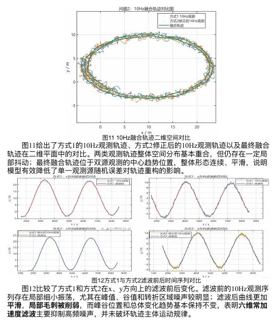
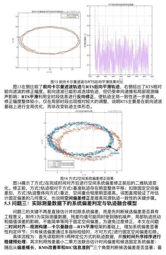
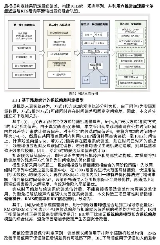
Read the first robot image like a detective. If two trajectories overlap in the wide path panel, zoom to the residual panel and check its unit. A route spanning hundreds of metres can make a one-metre error visually disappear in an overlay. The component-error plot should tell you whether east–west and north–south mistakes have different patterns. If errors spike during turns, revisit the motion approximation; if they remain shifted in one direction, revisit calibration. The figure supports a claim only when you say which pattern you expected and what the displayed pattern actually shows.

The second image compares a smoothed path with residual distributions. Ask whether the smoothing used later observations and whether the reported metric is for an offline reconstructed path. A smoother may visibly reduce jitter while also rounding a sharp turn. The residual distribution should show both central spread and tails; an attractive centre is not enough for tasks near distance boundaries. If a few positions are badly wrong, a 95th-percentile Euclidean error can matter more to the schedule than a small average RMSE.

The comparison table should keep dataset and baseline definitions in view. Do not put the noise-free attachment’s near-zero alignment discrepancy, the noisy attachment’s RMSE, and the field bias decision in one unlabeled “accuracy” column. They are different metrics on different conditions. A clear table can have rows for attachment and method, columns for time shift, retained bias, reference metric, and evaluation window. The caption should explain the units and which numbers are directly comparable.

From path to task windows

For targetat, calculate

$$
d_j(t)=|p(t)-q_j|2,\qquad
\theta_j(t)=\operatorname{atan2}(q{j,y}-p_y(t),q_{j,x}-p_x(t)).
$$

A task is feasible only when range, visibility, dwell time, and device constraints hold. Interpolate threshold crossings; a 0.1-second grid can distort short windows. Under path uncertainty, requireinstead of testing only the mean.

For equal-reward single-device intervals, earliest-finish selection is optimal. For heterogeneous photography durations, rewards, and turning restrictions, use binaryand possibly transition:

subject to overlap, window, and angular constraints. Distinguish the proof for interval scheduling from the solver certificate for the integer program.

Let us inspect one target with elementary geometry. Put the robot atmetres and a target atmetres. Their distance ismetres. If the shooting range is at most 5 metres, this point is exactly on the feasibility boundary. If the estimated robot-position ism, the distance becomesm and appears feasible. If the true-position ism, distance becomesm and appears infeasible. A small coordinate uncertainty, far smaller than many whole-path errors, changes the yes/no decision. This is why a path’s average RMSE does not certify each borderline task.

Now add a preparation rule: the robot must remain within range and below a speed threshold during the five seconds before firing. Checking only the position at the firing instant would miss a robot that entered the range during the last half-second. On a 10-Hz grid, five seconds contains about fifty intervals. Check each relevant sample, and pay special attention to entry and exit times between samples. Interpolating a threshold crossing can improve the estimate, but interpolation also has uncertainty; if the margin is thin, a conservative buffer or denser measurement may be more honest than a hundredth-of-a-second answer.

The displayed probability conditionis meaningful only after we have a calibrated distribution for position uncertainty at that time. RMSE alone is not a probability model. A two-dimensional covariance from the filter, validated against residuals, could support an approximate chance calculation; alternatively, use a declared worst-case position radius or sampled perturbations. State which approach is used and whether the requirement applies at one instant or across the whole preparation window. If it is across the whole interval, satisfying 95% at each separate grid point does not automatically give 95% joint-window feasibility.

After candidate windows are trustworthy, scheduling needs its own proof or audit. For equal-value, one-device intervals with no other conflicts, selecting the interval that finishes earliest and repeating has a classic optimality argument: any schedule can replace its first chosen interval with the earliest-finishing candidate without losing room for later compatible intervals. But add unequal rewards, two devices sharing a battery, or angle separation between repeated photographs, and that simple exchange may no longer apply. A binary optimization formulation or another justified method must encode the added rules. Do not transfer a proof from a simpler model to a richer one merely because both are called “scheduling.”

Even when a mixed-integer solver reports an optimal solution, verify the selected schedule independently. Recalculate each task’s range and full preparation-window speed and acceleration; recheck overlaps and angle differences; recompute the objective from selected rows. Compare the solver’s declared gap or certificate with the formulation it actually solved. A certificate for a flawed candidate set or missing rule is not a certificate for the physical mission. The body should make those scopes visible.

Geometric feasibility becomes explicit time windows.

The decision layer consumes the fused path and separates devices.

Show selected targets, directions, and conflicts spatially.

Scenario lines show whether the recommended schedule survives calibration change.

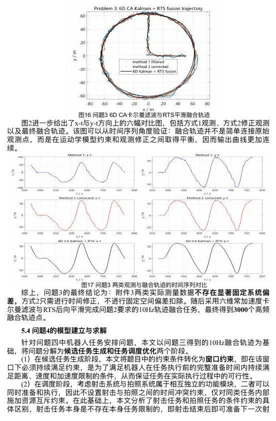
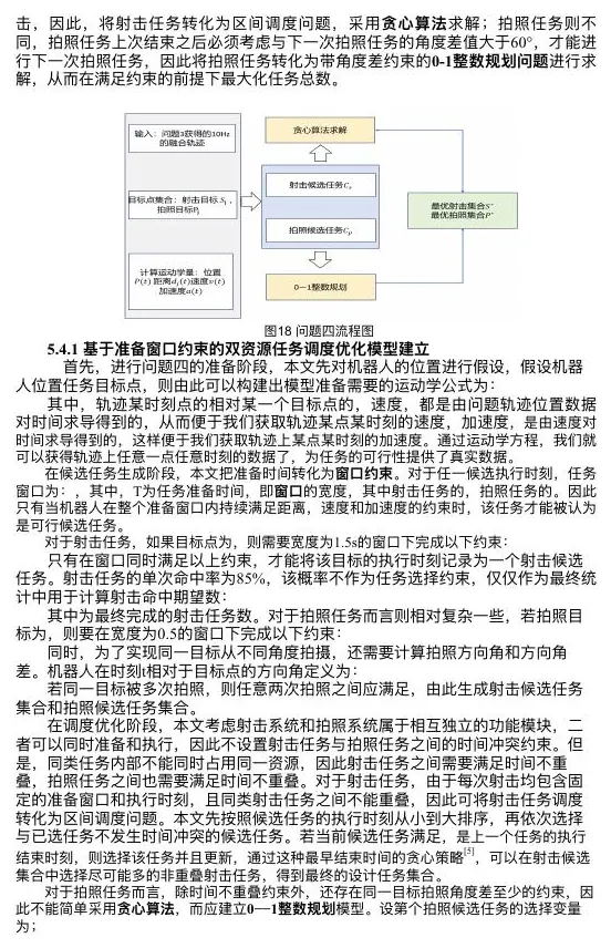
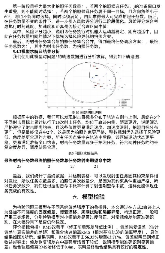
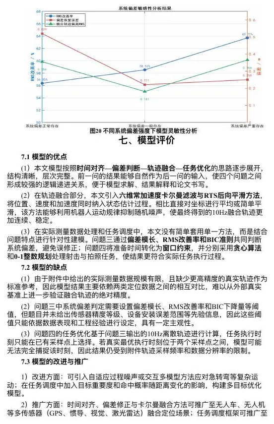
The window image should make it possible to check the whole preparation interval. If it marks only firing instants, ask where distance, speed, and acceleration were checked before those instants. The scheduling diagram should show separate shooting and photography resources and the angle rule for repeated photographs. The selected-task geometry should link target locations and viewing directions to the chosen time intervals; a spatial scene without time labels cannot verify non-overlap. Finally, the sensitivity image should put its perturbation unit and tested range on the axis. A line labeled merely “parameter change” gives no reader a way to judge whether the stressed values are plausible.

Choose one selected task from the figure and audit it. Find its target coordinate, final estimated position and uncertainty, full preparation interval, device resource, and any repeat-angle partner. Recompute its distance and motion checks. Then change the path by a small declared amount and see whether the task remains. This turns a four-image gallery into a connected explanation of how a location estimate becomes a conditional operational decision.

A path may look smooth while its task schedule violates a window. The matrix below forces us to test each output at the level where it is produced, rather than letting downstream polish hide an upstream mistake.

Pipeline validation matrix

Claim	Evidence	Stress test	Failure response
one offset synchronizes sensors	objective + block estimates	clock drift	affine/piecewise time map
fixed bias is real	held-out RMS + BIC	block resampling	keep no-bias model
fusion improves position	sensor baselines + innovations	noise and missing bursts	retune/change dynamics
windows are accurate	geometric replay	position/target perturbation	safety margins
schedule is useful	count, reward, utilization	duration/range/turn changes	robust alternative

Sensitivity as a decision surface

Vary clock offset, bias, sensor noise, maximum range, dwell time, and turning limit jointly. Rerun the whole pipeline and record both statistical metrics and selected tasks. A small RMSE change is harmless if the schedule is unchanged; a tiny calibration change that swaps many tasks is important.

Monte Carlo draws from calibration uncertainty estimate selection frequency. A target chosen in 99% of scenarios is a robust core; one chosen in 45% is conditional. This is more honest than one deterministic schedule.

Those 99% and 45% values are illustrative ways to read a selection-frequency plot, not measured frequencies from the supplied robot report. Imagine drawing 100 plausible calibration scenarios. If task A is selected in 99 and task B in 45, A is a strong candidate for a dependable core under the tested uncertainty model, while B is conditional. But ask why B comes and goes. Perhaps a small position shift moves its preparation window out of range; perhaps the angle rule makes it conflict with another photograph; perhaps an offset change changes when the robot passes the target. Different causes demand different remedies.

Plot a decision surface, not just an error surface. On one axis put clock offset, on another maximum allowed range, and color each grid cell by number of selected tasks or by whether task B is chosen. You may discover a sharp boundary: ats task B is valid, ats it disappears. If the calibration uncertainty spans both sides, quoting only the nominal 27-task schedule is risky. A table showing which tasks remain across several declared scenarios may communicate the same fact more clearly than a dense heatmap.

Do not vary a parameter in isolation when the fitted parameters are correlated. On a straight robot path, clock shift and along-path spatial bias can partially imitate each other. Drawingandindependently from separate intervals may create pairs that the calibration data do not support. Use a joint uncertainty estimate or test named physically plausible pairs, and say which method generated them. Re-run alignment, fusion or path perturbation, candidate generation, and scheduling as required. If you vary only the final optimization weights while freezing candidate windows, you have not measured sensor-to-task sensitivity.

For the bicycle policy, a decision surface could use expected station-1 demand and station-2 demand. In our tiny example, move two bikes when demands areunder the chosen cost. When station-2 demand rises, a smaller move may become safer. Mark the regions where move zero, one, or two is recommended. A manager can use that map to decide whether tomorrow’s forecast lies comfortably inside one region or close to a switching boundary. The boundary is more useful than one derivative of shortage at the nominal point.

Sensitivity ranges need justification. Ademand test may be a sensible classroom stress case, but a production plan should connect it to observed variability or a decision-maker’s concern. A-m target-coordinate perturbation may represent surveyed location uncertainty; a ten-degree camera-angle test may represent sensor calibration. If a range is arbitrary, label it as exploration. Do not write “the model is robust” simply because it survived one range chosen to avoid its failure.

Finally, interpret the surface in words: “Most tasks remain under the tested calibrations, but a small group near the range boundary is conditional; we recommend the stable core and require another location check before adding the borderline tasks.” That sentence ties a graph to an action. A rainbow sensitivity picture with no recommendation would leave the reader to decide why it mattered.

Consider a final miniature case that combines the chapter’s checks. A library manager must decide how many extra evening room-hours to staff during exams. The model predicts that extending two rooms by one hour each will reduce turn-aways. We have an optimizer’s recommendation, but we do not yet have an evidence-backed decision. First, verify the accounting: two one-hour extensions consume exactly two room-hours; no booking is assigned to a room outside its staffed interval; the objective is calculated from the model’s actual assignments. If the program reports three extra bookings in a room with only one extra hour and each booking lasts an hour, it has a constraint bug. We should catch that on a tiny hand-checkable timetable before reporting any percentage improvement.

Second, check whether the demand model describes the observed setting. Did arrivals actually cluster after closing during past exam weeks? Are some students turned away because rooms are full rather than because doors close early? If the historical turn-away count is zero at the extension hour, the proposed staffing may be feasible and optimally allocated under the model but irrelevant to the real shortage. Plot arrivals and occupancy by hour, and compare the model’s predictions with held-out evenings. This is validation against the world, not merely a repeat of the program’s internal arithmetic.

Third, compare with a baseline decision made from the same information. Perhaps the library normally keeps its busiest room open one hour longer and does not open a second room. Test that policy and the proposed policy on identical held-out evenings. Report both turn-aways and staff-hours. If the proposed plan prevents one extra turn-away but needs twice the staffing, the decision maker may not prefer it. The baseline forces us to translate “improved model score” into a relevant operational trade-off. We cannot change the baseline after seeing which policy wins.

Fourth, stress the recommendation. A late exam announcement might double arrivals during the final hour. If the model then recommends a different room, identify the switching point. Or one staff member may be absent, leaving only one room-hour available. Does the recommendation degrade gracefully, or does it become infeasible because we wrote a hard requirement that cannot be met? We should present a fallback in the result discussion. A decision meant for tomorrow must survive more than the exact historical average.

You can now see why the four checks are nested rather than interchangeable. The timetable can pass program verification and fail historical validation. It can match historical arrivals and still lose to a cheap baseline. It can beat the baseline on ordinary evenings and fail under exam-week surge. Each check answers a new question the earlier one could not. This is the continuity we want in a results chapter: not four detached boxes, but an increasingly demanding test of the same proposed action.

The language of the final recommendation should reflect that progression. I might say, “On the recorded exam-period evenings, extend the two busiest rooms by one hour each only when late arrivals exceed the observed switching threshold; in the tested timetable this avoids more turn-aways than the existing one-room extension at the same two room-hours, but the policy should be rechecked if a room becomes unavailable.” This is an illustrative wording, not a fabricated empirical result: the article has not supplied an actual library dataset or a measured threshold. Its value is grammatical. It states an action, population, comparator, cost, and condition. Once real data exist, replace the conditional language with the actual measured values and cite the supporting table.

The library example also reminds us that some validation outcomes are behavioral. Students may arrive earlier once they know rooms stay open, so past arrivals are not necessarily the arrivals under a new policy. A retrospective replay estimates what the change would have done under yesterday’s behavior; it does not prove what people will do after the schedule changes. This is a limitation we should name precisely rather than hiding behind “more research is needed.” A small trial or updated arrival monitoring would directly address it.

We end where we began: a result is not credible because it has many decimal places. It is credible when the rule was implemented correctly, the important mechanism matches observations, the proposed decision beats a fair alternative on the relevant measure, and the recommendation’s boundary is visible. That is exactly the mindset to carry into optimization. The next lesson’s profit or cost optimum will be a candidate decision, not the end of the evidence chain.

We can now enter optimization with a better question than “Did the solver finish?”: do the variables match the decision, do the constraints match reality, and would the proposed action survive the same evidence and stress checks we have just used?