Mathematical Modeling 1 - From Reality to a Model

Imagine a commuter who is usually picked up at 6:00 p.m. Today he arrives thirty minutes early, walks toward home, meets the car on the road, and gets home ten minutes ahead of schedule. How long did he walk? Write down a guess before you look for a formula. We know neither driving speed nor walking speed. That is exactly why this is a good first modeling question: the right relationship may matter more than the missing numbers.

I want to build this course the way we would work at a board together. I will pose a concrete problem, let you predict, say what we are assuming, make the smallest calculation that can answer it, and ask what observation would overturn the result. The commuter is only our first puzzle. We will also ask how a restaurant should replace dishwater, how a traffic signal gets its timing, and how a campus manager can staff a dining hall. Across all four, the common skill is turning a vague situation into a testable question.

Mathematical modeling is not the act of attaching a fashionable algorithm to a dataset. It is the controlled replacement of a real system by a simpler mathematical object that is useful for a stated decision.

Our commuter guess already contains the first modeling question: what exactly are we trying to determine? Before solving any of the four examples, let us name the choices we will make in every one of them. Later, when the equations arrive, you can check whether each choice still matches the story.

The modeling contract

A model must make five things explicit:

1. Purpose: What decision, explanation, or prediction is required?
2. Boundary: Which objects, time scales, and interactions belong to the system?
3. State: What quantities are sufficient to describe the system at a given moment?
4. Mechanism: How do those quantities interact or change?
5. Evidence: What observation could show that the model is inadequate?

This contract prevents a common failure: solving a mathematically interesting problem that is not the problem asked.

Let us make those five items less like a checklist and more like a conversation. If I say, “The campus shuttle is bad,” you cannot solve that sentence. Ask me what I mean. Maybe I miss my 9:00 class, maybe the average ride is slow, maybe evening riders have no service. Those are different purposes and could lead to different recommendations. Say I answer: “I need to decide whether to add one shuttle at 8:30 so that at least 90% of riders reach the classroom before 9:00 without exceeding the vehicle budget.” Now we have a decision and an observable success condition.

Next ask where the system begins and ends. Do riders arrive at a stop, board a bus, travel, walk from the drop-off point, and enter the classroom? If the target is arriving at class by 9:00, the last walk belongs in the boundary. If we count arrival at the bus stop as success, our model will give an answer to the wrong clock. We might ignore the rider’s breakfast or what happens after class; those may not affect this decision. Write what you excluded, because somebody reviewing the recommendation will otherwise have to guess.

Now imagine a clock at 8:35. How much do we need to know to predict the next five minutes? Perhaps the number of people waiting at each stop, shuttle locations, free seats, and travel conditions. These are candidates for the state. Not every detail of every student’s day is needed. But omitting the number of waiting riders would make it impossible to represent a queue. The test of a state is whether it contains enough of today’s situation for your declared next-step rule to work.

What changes that state? Riders arrive; shuttles reach stops; passengers board until seats fill; buses leave; travel times pass. That story is the mechanism. We might start with fixed arrival and travel rates. We would not claim they are permanent facts; they are a simple baseline. If rain delays travel and increases arrivals, we must either include rain as an input or declare that the recommendation is for ordinary dry mornings only.

And how would we know if the model is wrong? Record real arrival times at classes over several mornings, not just how accurately we predicted buses reaching the last stop. Compare the fraction of riders reaching class before 9:00 with the predicted fraction, and inspect bad mornings. That is evidence tied to the original purpose. The five items now form one coherent question: what choice do we need, what events affect it, what quantities track those events, how do they evolve, and which observation could disprove our recommendation?

For a first experiment, take a tiny stop with ten riders at 8:30, a vehicle with eight empty seats arriving at 8:35, and another vehicle arriving ten minutes later. If everybody needs to be in a classroom five minutes after drop-off, eight can catch the first shuttle and two cannot. You do not need a simulation to see why seat capacity matters. If a program says all ten catch the first shuttle, the tiny scenario immediately reveals a missing constraint. After your smallest example works, add several stops, uncertain arrivals, and real travel times. A beginner who can diagnose a ten-person example is better prepared for a thousand-rider dataset than one who starts by importing a sophisticated solver.

The shuttle example gave us five questions to ask about a system. Let us now apply them to a very different one—a basin of water in a restaurant. If the same questions still help when the physical mechanism changes, they are useful modeling habits rather than a checklist tied to one problem.

Start with a question, not an equation

Imagine you own a small restaurant. Before lunch, you fill a basin with hot water. A worker rinses each dirty plate in cold water and then dips it into this basin. The water must stay warm enough to clean the plates, but it cannot be so hot that the worker burns their hands. Refilling and reheating cost money. How many plates can this one basin handle before you should replace the water?

You might answer “a hundred” or “a few hundred.” Good: write down your guess. Now tell me what would actually make the basin unusable. Is it that a fixed number of plates has gone through it, or that the water has cooled below a temperature you consider acceptable? The second answer suggests something we can measure after every plate: the water temperature. We call that changing quantity the state of the system. The number of plates is an output we infer from the state; it is not what controls the temperature.

There is a second complication. Dirty plates can make the water unhygienic even while it is warm. So the temperature model below answers only the thermal part of the question. In a real restaurant, test both the temperature threshold and water cleanliness, and replace the water when either requirement fails. I am telling you the limitation before doing the calculation because otherwise an impressively precise plate count would give you false confidence.

Draw the boundary in your head

Take the basin and the plate currently being dipped as your system for one washing step. The water begins at temperature; the plate, after the cold rinse, begins at. We expect the warmer water to give up energy and the colder plate to gain it. If we assume that one dip is fast, heat lost to the surrounding air during that dip is small. If we assume the basin is well mixed, we can represent all its water by one temperature. Neither assumption is automatically true. They make a first calculation possible and tell us what to check later.

“Energy lost by the water equals energy gained by the plate” is the balance for this boundary. Letbe the mass of water in kilograms,the heat capacity of water in joules per kilogram per degree Celsius,the mass of one plate, andits heat capacity. If both reach the same temperatureafter the dip, the equation is

Read the left side in words: kilograms of water times energy needed to change one kilogram by one degree times the degrees by which it cooled. The right side says exactly the same thing for the warming plate. Both sides have units of joules. Notice that I did not begin with an algorithm. I began with the heat-transfer story, chose a boundary, and then wrote what must balance across it.

Solve this one-line equation for the new water temperature:

This weighted average immediately passes two sanity checks. If the plate has almost no mass,approaches zero and the water barely cools. If we keep increasing the plate’s thermal mass, the final temperature moves closer to the plate’s starting temperature. If your computation predicts a temperature higher than both starting temperatures, it has a sign or implementation error.

Let us put in illustrative numbers

Suppose the basin holds 20 kilograms of water, initially at. Set the minimum acceptable temperature to. For a first approximation, use. Suppose each plate weighs, its effective heat capacity is, and it enters the hot basin at. These are teaching numbers, not measurements of your restaurant. Before trusting the answer, weigh actual plates, measure how much water is in the basin, and record temperatures before and after a few dips.

Hereand. After the first plate,

The tiny drop makes sense: the water has far more thermal capacity than one plate. But do not multiply this first temperature drop by the number of plates and assume it remains constant. As the water cools, the difference between water and the next cold plate becomes smaller; every subsequent plate takes a slightly different amount of heat.

We can repeat the update by hand for a few plates or compute it in a loop. To understand the answer before running code, subtract the plate temperaturefrom both sides. With

the recurrence becomes. Afteridentical plates,. The basin remains above the threshold while

Taking logarithms, remembering thatis negative and therefore reverses the inequality when we divide by it, gives. That is roughly 205 plates for these illustrative numbers. The 206th plate takes the water below our declared threshold. Whether you count a plate washed at exactly the threshold as acceptable should be written down before you round your answer.

Could we have estimated the count more crudely? The basin can lose aboutmillion joules before reaching the threshold. If every plate required exactlyjoules, we might divide and say 278 plates. But a plate dipped when the water is still nearabsorbs more than 6000 joules. That 278 is an optimistic upper-bound-style estimate under this simplified setup, not the answer to the mixing model. The disagreement between 278 and 205 teaches us why a changing state needs a step-by-step model instead of one division.

What would change the recommendation?

Keep the physical question in view. If a heater runs continuously, energy enters the basin; if the room is cold, energy leaves the basin between plates; if plates are different sizes, each dip transfers a different amount of energy. A convenient general statement is

Now that the terms each name a real event, you can decide which to include. If heating is turned off and thirty plates are washed quickly, perhaps room loss is negligible over that short interval. If plates are washed over two hours, it might dominate. A thermometer reading after every tenth plate and a clock can tell us. That is a test of an assumption, not an invitation to add complexity for its own sake.

Finally, check units wherever you go. The quantitiesandare both energies; we may equate them. We cannot add a temperature directly to an energy, and we cannot put a quantity measured in joules inside an exponential without making it dimensionless first. Unit checks are cheap, and in beginner models they catch a surprising number of expensive mistakes.

Turn the basin calculation into an actual experiment

If you were standing in that kitchen, what would you measure first? Put a graduated mark on the basin so you can estimate the water volume. Water’s density near these temperatures is close enough to one kilogram per litre for a rough classroom estimate, so a twenty-litre fill suggests about twenty kilograms; for a careful calculation, record or measure the actual mass. Put a thermometer in the same representative location each time, stir gently, and record the starting temperature. Weigh a sample of plates instead of using my teaching number. Keep track of what kind of plate is being washed and whether the plate was room temperature or just rinsed in colder water.

Now make a table with columns for dip number, elapsed time, water temperature before the dip, water temperature after the dip, plate type, and whether a heater was on. Ten well-recorded dips can already reveal useful patterns. If the temperature drops by aboutfor the first ordinary plate, our first illustrative update has the right order of magnitude. If it drops by a full degree, something in the teaching values or in the model of one dip is wrong. Perhaps the dish is heavier, cold water stays on it, hot water is removed with it, or the basin contains less water than we assumed. Do not “fix” the answer by arbitrarily changing a parameter until you know which mechanism caused the discrepancy.

How would you separate plate cooling from loss to the room? Leave the basin untouched for the same amount of time it would take to wash ten plates, and record how much it cools. That gives a control experiment. If it loseseven without plates, then some observed drop during washing is environmental. If it barely cools, the plates probably dominate over that interval. This is the most approachable version of an experimental control: compare a condition with the hypothesized cause to one without it.

What about the cleanliness requirement we set aside? Ask the staff what threshold actually governs replacing the water—temperature, visual dirtiness, a sanitation rule, time in use, or a combination. A thermal count of 205 plates is not a sanitation recommendation. If water is cloudy after 40 plates, the real operational limit could be 40. If plates are cleaned by detergent and hot water is refreshed continuously, the kitchen’s procedure may have a different limiting mechanism entirely. A model’s purpose is to guide a real decision, so measuring the actual stopping rule is part of the mathematics.

Try turning the calculation into a recommendation with uncertainty rather than a single number. Suppose your measurements suggest the basin stays within the temperature range for somewhere between 170 and 230 plates under typical shifts, but water cleanliness triggers replacement between 90 and 120. The practical recommendation is not “the model says 205.” It is “schedule replacement after at most about 90 plates under these observations, and verify hygiene requirements separately.” We would also explain how the range was obtained, how many shifts were measured, and why it may fail on a colder or longer shift. The conclusion changed because we finally asked the full restaurant question rather than only the easier thermal one.

You might be tempted to make the model more detailed than the data support. We could write spatial heat-flow equations for every layer of water, model detergent chemistry, and estimate the thermal properties of each plate. But if staff replace the water after 90 plates due to dirtiness, refining the thermal estimate from 205 to 201 plates will not change the action. This is a good point to stop. An elaborate model is not intrinsically a better model; it is better only when it makes a materially different, testable decision possible.

One final practice question: imagine the basin is half as large but starts at the same temperature. Would the plate limit simply halve? In the constant-per-plate energy shortcut, it would. In the recurrence, the ratioalso changes, so the exact count is not necessarily half to the nearest plate. Predict that the limit decreases substantially first, then calculate it. If you can explain the direction without touching a calculator, you have understood the mechanism; the calculator supplies the precise value afterward.

We have just turned “How many plates?” into a changing temperature and an energy balance. Many modeling questions are not about heat at all: they ask us to assign, schedule, or choose. The next step is to translate those ordinary action words just as carefully as we translated the restaurant’s question.

Translate language into structure

Turn nouns into sets or parameters, verbs into decisions, and qualifiers into constraints.

• “Assign workers to tasks” suggests binary variables.
• “At most one” becomes a sum bounded by one.
• “Minimize total time” becomes an objective over selected decisions.
• “For every day” creates a time index.
• “Uncertain demand” requires scenarios, distributions, or uncertainty sets.

For every subproblem, write an input–output sentence: “Given ___, estimate/choose ___ so that ___.” This small step often reveals dependencies between questions and prevents circular reasoning.

Let us translate an ordinary staffing request without skipping any steps. A manager says: “I have four workers and three stations—payment, food preparation, and pickup. At lunchtime each station must have at least one worker. Where should the fourth worker go so that customers wait less?” At first, the manager does not have an objective function. She has people, stations, a staffing rule, and a wish.

Draw four little circles for workers and three rectangles for stations. Connect workerto stationif they can be assigned there. Letwhen workeris assigned to station, andotherwise. Why only zero or one? In this half-hour snapshot, we are choosing a whole assignment; we are not asking a worker to beof a person. For each worker, the sentence “exactly one station” becomes. For each station, “at least one worker” becomes. These equations do not yet minimize waiting; they simply prohibit plans the manager cannot implement.

Now ask for service rates. Suppose the second worker at payment increases payment capacity from 25 to 50 customers per half hour, while a second worker at preparation increases its capacity from 40 to 70. If 60 customers arrive and pickup serves 80, allocating the spare worker to payment raises the three capacities to; preparation is still the bottleneck at 40. Allocating the spare worker to preparation makes them; payment is now the bottleneck at 25. Neither plan can handle all 60 arrivals in this oversimplified steady-state example! This is a useful discovery: the manager might need a fifth worker, a changed service process, or a temporarily different objective. Optimization cannot conjure capacity the system lacks.

Keep two columns labeled question and mathematical representation. “Can every worker serve every station?” goes beside the allowed edges of the assignment graph. “Must pickup always be staffed?” goes beside. “How much does moving a worker improve waiting?” goes beside measured service times and a queue model. A sentence with no representation warns that you may have ignored part of the problem; a variable with no originating sentence warns that you may be optimizing something nobody requested.

When a prompt has multiple numbered tasks, do not assume the numbers are independent. A forecast of lunchtime arrivals may feed the staffing decision; staffing may feed a cost calculation; those results may feed a recommendation. Make an arrow diagram and label each arrow with what it passes. If the recommendation uses a 12:30 forecast calculated from a feature that is only known after 12:30, you have built a loop through the future. This dependency diagram exposes the mistake before code turns it into a mysteriously excellent accuracy score.

The assignment equations made the manager’s rules explicit, but the capacities we used were estimates. The basin calculation likewise depended on a well-mixed tank and identical plates. How do we decide which simplifications are safe to keep and which ones might reverse the recommendation? That is the job of assumptions.

Assumptions are controlled approximations

A useful assumption removes complexity while preserving the mechanism that controls the answer. Classify assumptions as:

• Structural: interactions, independence, network topology, or state definition;
• Parametric: constants, bounds, distributions, or rates;
• Operational: resource availability, policy, timing, or implementation rules;
• Measurement: noise, missingness, resolution, or sensor bias.

Every important assumption should have a reason and a consequence. “Travel speed is constant because the route is short and uncongested; therefore travel time is proportional to distance.” A list of unsupported assumptions is decoration, not modeling.

Return to the basin for a concrete test. We treated the water as one perfectly mixed volume. This means a thermometer near the surface and one near the bottom should report roughly the same temperature, especially just after a plate is dipped. If they reportand, our one-temperature state is a poor description. A sensible extension might use two layers, but the measurement is what justified the extra state. Do not start by inventing layers without checking whether stratification matters.

We also pretended that all plates weighkg and arrive at. Those values may be roughly right for one kind of dish, but a metal baking tray and a light ceramic saucer will not absorb the same heat. Record plate types, frequencies, and approximate thermal masses. For a mixed stack, run the same recurrence with a differentfor each dip. If order is unknown, run several plausible sequences or sample them from observed frequencies. This is how a static toy model grows into an uncertainty analysis without losing the mechanism you already understand.

An assumption ledger is a way to keep promises visible. Put “well-mixed water” in one row, “equal plate thermal mass” in another, and “heater off during the wash” in a third. Beside each, record what makes it plausible, which part of the answer depends on it, and what observation could reject it. If the heater was running, our predicted 205 plates could be far too low. Add measured heater power in watts (joules per second) and the time between plates. Then power times time is energy entering the basin, with the same units as the heat transferred to plates. A unit check now tells you how to incorporate the new mechanism.

Not every assumption needs an elaborate sensitivity plot. If the restaurant only needs to know whether one basin survives 80 plates in a short lunch shift, even a much lower stressed estimate might exceed 80. The decision could be robust. If it needs 200 plates, small changes in heat loss or plate mix may push the answer across the threshold. The level of modeling effort should depend on how close the real decision is to the predicted boundary.

Once assumptions are visible, we can avoid two opposite mistakes: doing nothing because the real world is messy, or building an enormous model before we know what matters. Begin with the smallest calculation that respects the main mechanism, and add detail only when an observation shows why you need it.

Solve the simplest credible model first

Build models in layers:

1. a transparent baseline;
2. one extension that addresses the baseline’s largest failure;
3. a comparison showing whether the extension matters.

If a linear model answers the decision robustly, a deep network is not automatically better. Complexity must purchase predictive accuracy, realism, computational tractability, or decision quality. Report that purchase explicitly.

For our basin, the transparent baseline is the no-heater, well-mixed recurrence. The first extension is not “replace it with machine learning”; it is “measure cooling even when no plates are dipped, and account for that loss between dips.” Put a thermometer in the basin, leave it untouched for ten minutes, and watch the temperature fall. If it falls fromto, room loss may be tiny over a fast batch. If it falls to, it is too important to ignore. The more complicated model earns its place only if this difference alters the plate-count decision.

For the dining hall, a baseline is the demand-capacity balance. An extension could preserve individual arrival times and service-time variability in a discrete-event simulation. You need not know the name to grasp the idea. Keep a clock and a list of customers: when someone arrives, assign them to a free worker or make them wait; when a worker finishes, take the next customer. Repeating the clock events produces each person’s wait. Compare predicted waits with real lunchtime observations. If the simulation changes the suggested staffing pattern during peaks, the extension solved a real limitation. If both models agree across the observed range, the simple balance might be sufficient for the manager’s current decision.

The basin recurrence and dining-hall capacity balance gave us answers under declared assumptions. Neither answer is evidence that the kitchen or campus will behave exactly as predicted. We now need to test the whole path from story to code to decision, not merely admire the final number.

Validate the chain, not only the final number

Validation has several levels:

• implementation: does the code solve the equations written?
• internal: do units, bounds, conservation laws, and limiting cases hold?
• empirical: does the model reproduce held-out or historical observations?
• comparative: does it improve on a baseline under the same test?
• decision: would plausible uncertainty change the recommendation?

The final report should close the loop: questionabstractionsolutionevidencedecision. COMAP describes mathematical modeling competitions as an unscripted combination of modeling, problem solving, and writing; the deliverable is therefore an argument, not just a program (official MCM/ICM instructions ).

Let us validate the shuttle calculation one level at a time. First, implementation: set the toy stop to ten riders and eight available seats. Does your program leave two behind? If not, the boarding rule in the code contradicts the rule in your story. This check is often called verification. It does not prove the real shuttle system is modeled well; it proves only that your program carried out the declared rule on a case you understand.

Second, internal plausibility: a shuttle with eight seats cannot board nine people; predicted classroom arrival cannot be earlier than boarding; the number of riders waiting next minute should equal those already waiting plus new arrivals minus riders who boarded, assuming no one walks away. These are conservation, capacity, and chronology checks. You can catch impossible outputs even without collecting more data. A program that runs without errors can still violate all three.

Third, comparison with the world: collect several ordinary mornings of arrival, boarding, travel, and classroom timestamps. Fit any parameters on some days and test predictions on other days. Why not use the same days for both? Because a model can learn the quirks of the days it saw and still fail next Tuesday. If you use the actual travel time of the test-day shuttle as an input to a prediction that should have been made at 8:30, you have also leaked information from the future. Check what the dispatcher could really have known at decision time.

Fourth, comparison with a baseline: suppose the current schedule gets 78% of riders to class by 9:00. Your new plan predicts 92%. Test both against the same arrival scenarios, vehicle budget, and measurement definition. If the new plan needs another vehicle beyond the budget, the 92% is not a feasible improvement. If the old plan’s 78% was measured on rainy days and the new plan’s 92% on dry days, the comparison is not controlled. A useful baseline can be plain and imperfect; it must nevertheless be tested fairly.

Fifth, decision stability: what if travel time is five minutes longer than measured last week? Does the new plan still deliver at least 90% on time? What if arrivals at the busiest stop rise by 20%? You do not have to guess blindly. Change one input, rerun the calculation, and explain which riders miss the target. If a small plausible perturbation makes the recommendation fail, present the recommendation as conditional and consider a spare shuttle, an earlier departure, or another route. This is sensitivity analysis in the service of a real decision.

Finally, write the result for the person who asked. “Assign one additional eight-seat shuttle to the 8:35 stop arrival, subject to the vehicle budget; on held-out ordinary mornings the predicted on-time fraction rises from 78% to 92%, but the plan falls below 90% when travel is more than five minutes slower.” This is an illustrative sentence, not a measured result from Columbia’s shuttles. It shows what a conclusion ought to contain: an action, a metric, a comparison, the operating range, and the main failure condition. A bare “accuracy = 92%” does not tell the dispatcher what to do.

If you are new to mathematics, you may worry that these checks make every answer uncertain. They do, in a healthy way. Modeling does not mean being afraid to conclude anything; it means knowing which conclusions are earned. Our commuter answer is exact under a clear symmetry assumption. The two-day theorem guarantees an existence result under continuity but not the location. The basin’s plate count is conditional on measured thermal values and stopping rules. The shuttle recommendation can be supported by held-out mornings but still need stress testing for rain. Different problems give different kinds of certainty, and good teaching should not pretend they are all the same.

The shuttle validation example was deliberately long. On a live problem you need a compact way to notice a missing decision variable, an unmeasured input, or a test you forgot to design. Use the following questions as a pause before moving from formulation to computation.

Working checklist

Before proceeding, be able to answer:

• What is the decision variable or predicted quantity?
• Which data are observations, and which numbers are assumptions?
• What baseline can be solved today?
• What failure mode motivates the next layer?
• Which figure or test will support the conclusion?

If any answer is vague, the model is not ready for optimization.

You have seen a restaurant, a shuttle, and several short definitions. Let us slow down and build one campus decision from its very first sentence. The dining-hall case will let us use the checklist while the variables and constraints are still small enough to check by hand.

The dining hall: a model from scratch

Suppose a university wants to reduce the waiting time at a campus dining hall without increasing the weekly labor budget. This sentence is still a situation, not a mathematical problem. We must decide who acts, what can be changed, what cannot be changed, and what “better” means.

Step 1: write the decision sentence

Use the template introduced earlier:

Given predicted customer arrivals, service times, worker availability, and labor costs, choose the number of workers assigned to each station in each 30-minute period so that expected waiting time is minimized while the labor budget and staffing rules are respected.

The nouns now become mathematical objects. Letbe the set of time periods,the set of stations,the expected arrival rate,the service rate of one worker at station, andthe number of workers assigned to stationduring period. Notice thatis a decision, whereasandmust be measured or estimated.

Step 2: draw the system boundary

The boundary might include arrival, ordering, payment, food preparation, and pickup. It might exclude where students go after collecting food. A boundary is neither correct nor incorrect by itself; it is useful when it contains the mechanisms that dominate the target quantity. If pickup congestion blocks the preparation station, pickup must be included. If it never blocks upstream work, it can initially be omitted.

Write a unit beside every quantity. For example,has units customers/minute,has units customers/(worker·minute), andhas units customers/minute. A utilization estimate

is dimensionless. If, demand reaches or exceeds nominal capacity, so a stable steady-state queue should not be expected. This one calculation is already a useful baseline.

Step 3: separate data from assumptions

Arrival timestamps, transaction durations, and schedules are observations. “Service times are independent” and “one worker has a constant service rate within a period” are assumptions. Estimate an empirical distribution rather than reporting only the mean: a mean of two minutes can hide a mixture of many 30-second orders and a few ten-minute orders.

Make an assumption ledger with four columns: assumption, reason, consequence, and test. The constant-rate assumption may be reasonable over a short interval; its consequence is a simpler queue; its test is whether the rate changes systematically within that interval. An assumption that cannot be connected to a consequence is probably too vague.

Step 4: construct a baseline and one extension

The baseline assigns enough workers to keep estimated utilization below a chosen threshold such as. It ignores random variation but is transparent. The extension uses a queueing approximation or discrete-event simulation to estimate the waiting-time distribution. Compare both under the same arrival scenarios. If both recommend the same staffing pattern, the simpler model may be sufficient. If they differ during sharp peaks, the extension has identified where variability matters.

Step 5: decide what would falsify the model

Reserve several days for evaluation. Compare predicted and observed queue length, mean wait, 90th-percentile wait, and the fraction of periods exceeding a service target. Inspect errors by weekday and time of day. A model that is accurate at noon but fails at closing time has a defined operating range, not universal validity.

Your first deliverable

Create a one-page specification for a real system around you. It must include one decision sentence, a boundary diagram, a variable table with units, three assumptions with tests, one baseline, one extension, and two validation metrics. This exercise is deliberately algorithm-free: the purpose is to learn that formulation comes before computation.

Work one dining-hall period on paper

That specification can feel abstract, so let us pretend we are standing beside the dining-hall manager at 12:00. In the next half hour, past records suggest that about 60 customers will arrive at the payment station. One worker can serve about 25 customers per half hour under ordinary conditions. The manager can assign either two or three workers. Which arrangement would you try first? Make your own prediction before using a formula.

Two workers can serve about 50 customers in half an hour. If 60 arrive, a rough balance says the queue grows by 10 customers even if it was empty at the beginning. Three workers can serve about 75. In the same rough balance the station has capacity to absorb the 60 arrivals; the queue need not grow. The calculation is not a proof that nobody waits. Customers can arrive in a burst while servers happen to be busy. It is a first way to reject a clearly overloaded plan.

Express the same idea in units. At 60 customers per 30 minutes, the arrival rate iscustomers/minute. Each worker’s service rate iscustomers/minute. With two workers, nominal capacity iscustomers/minute and. With three, capacity iscustomers/minute and. The numberis called utilization: it compares demand with capacity, and has no unit because the units cancel. A value over one is warning of persistent overload if the rates stay like this. A value below one leaves spare average capacity but does not guarantee a short wait during peaks.

Do you see why we wrote the 30-minute balance before saying “use queueing theory”? The manager’s first question was whether the extra worker is plausibly necessary. The elementary balance answers that much without a distribution, a simulation, or a specialized library. If the team needs to know whether the 90th-percentile wait is below five minutes, the balance does not answer enough: it is time to model the variability of arrivals and service times. The need for a sharper answer, not our appetite for sophisticated mathematics, tells us when to extend the model.

We have also hidden a decision trade-off. Perhaps three workers at payment leave only one worker preparing food, so the bottleneck simply moves. Before the manager acts, the boundary must include other stations and the total labor constraint. If a worker costsper hour, adding one for a half hour costs. Compare that cost with measured waiting and with the cost of longer waits. Without some valuation or a hard wait-time target, the phrase “optimal staffing” is unfinished: optimal with respect to what?

Try a quick counterexample. Suppose 30 of the 60 customers arrive within the first five minutes. Three workers’ average capacity of 75 per half hour sounds generous, yet during those five minutes they can serve only aboutcustomers. A temporary queue of roughly 17 or 18 people forms. A model based only on total half-hour arrivals will miss this burst. You can test the constant-arrival assumption using timestamps, not by adding a vague sentence to the limitations paragraph.

If those timestamps exist, create two plots: cumulative arrivals against cumulative service capacity, and observed wait against predicted wait across several days. The gap between the two cumulative curves is an approximate queue. Measure whether errors cluster at lunch peaks; if so, shorten the time periods or use a stochastic queue. If predicted and observed waits agree under ordinary conditions but not at the first five minutes of lunch, report that precise operating range. A model that identifies its own weak spot is far more useful than one that prints a single unqualified staffing schedule.

Data, choice, and rule are different kinds of quantities

Let me spell out a distinction that beginners often learn only after a solver gives nonsense. The 60 arrivals are an observation or forecast: we do not get to change yesterday’s timestamps. The number of assigned workers is a decision: the manager can choose it within staffing rules. Thecost is a parameter computed from wages and time. A sentence like “no more than three workers at payment” is a constraint on decisions. A queue of 18 at 12:05 is a state of the system, created by earlier arrivals and service. These labels are not ceremonial. They tell us which quantities can be optimized and which must be estimated.

You can test your understanding by changing only one quantity at a time. If arrivals increase to 75 while staffing remains at three, utilization becomesand the average spare capacity vanishes. If the manager assigns four workers with arrivals still at 60, utilization falls tobut labor cost rises. If service capacity of one worker falls to 15 customers per half hour because of a slow register, three workers provide only 45; the queue grows despite a staffing number that looked fine yesterday. Every change corresponds to a different real-world intervention or failure, so do not silently treat it as the same scenario.

At this point, I would ask you to explain the case to a classmate without any Greek letters. You should be able to say, “Customers arrive faster than two workers can serve them, so a line builds. A third worker gives average breathing room, but a lunch rush can still create a line. We would check arrival timestamps and the other stations before changing the schedule.” If you can say that, the mathematical symbols have done their job: they clarified a decision rather than replacing it with jargon.

The dining hall was a full workflow: decide, calculate a baseline, and test it. The opening slides use four shorter puzzles to sharpen individual habits. We will take them one at a time—an invariant, a continuity argument, a safety-timing calculation, and an energy balance—then ask which habit each one contributes to the longer workflow.

Lecture casebook: four problems before any algorithm

The opening lecture deliberately begins with ordinary situations. Each one teaches a different modeling habit. Work through them before reaching for a solver.

The early commuter

A commuter is normally picked up at the station at 6:00 p.m. One day he arrives at 5:30, does not phone his wife, and walks toward home along her usual driving route. She leaves at the usual time, meets him on the way, and they arrive home ten minutes earlier than on a normal day. How long did he walk? Before reading the answer, choose a number. A lot of people immediately say “thirty minutes,” because he arrived thirty minutes early. But that would require his wife to meet him exactly when she normally reaches the station; she meets him on the road, so he stops walking before then.

What information do we know about the car? We do not know its speed, the distance from home to the station, or the man’s walking speed. Surprisingly, we do not need them if the wife’s speed along the route is the same on the outward and return drives. Imagine the segment from the roadside meeting point to the station. On an ordinary day, she drives that segment toward the station and then the same segment back with her husband. On the unusual day, she skips it twice. The total driving time saved is ten minutes; hence each skipped traversal would have taken five minutes.

The meeting must therefore occur five minutes before her normal 6:00 arrival, at 5:55. The man started at 5:30 and walked until 5:55: he walked 25 minutes. Check the clock calculation explicitly:minutes. The structure, not a measured speed, carried the answer.

Let me ask you to challenge it. What if the wife speeds up on the way home, or the road is one-way and the return route differs? Then the two saved traversals are no longer equal, so “five plus five” need not hold. What if she gets the news and leaves early? Then her departure schedule has changed, and the usual reference clock no longer works. The conclusion is conditional, as a model’s conclusion should be.

This is a lesson about invariants: a property that remains usable even when other numerical details are unknown. You can model the full positionsand, introduce two speeds and a distance, and solve a system of equations. You could also notice the two skipped road segments and solve the problem in three lines. Simplicity here is not laziness: it exposes exactly why the answer is determined.

The two-day journey

On Monday, a walker sets out from villageat 9:00 a.m. and reaches villageby 5:00 p.m. On Tuesday, the same walker starts atat 9:00 a.m. and returns along the same path toby 5:00 p.m. Must there be a point on the path where the walker was at the same clock time on both days? You need not know whether either day’s speed is constant. The walker might pause, accelerate, or even backtrack. Take thirty seconds to imagine both journeys before following the proof.

One wonderfully concrete way to see it is to imagine two copies of the walker traveling simultaneously on the same path: Monday’s copy walks fromto, Tuesday’s copy walks fromto. At 9:00 the copies are on opposite ends. By 5:00 their ends have exchanged. If neither teleports and they stay on the same continuous path, they cannot exchange order without meeting. Their meeting point is exactly the position occupied at the same clock time on the two real days. The story is a proof, not a numerical prediction of where they met.

If you want mathematical notation, measure distancefromalong the route. Set. At 9:00,is negative: Monday is at(), Tuesday at(), so. At 5:00 it is positive: Monday atand Tuesday at, so. The intermediate-value theorem says a continuousthat changes sign must take the value zero at some time. At that instant the two positions coincide.

Why did I state the starting and ending clock times? If Tuesday’s trip happens between midnight and 8:00 a.m., it need not share a time interval with Monday’s trip, so “same clock time” has a different meaning. If the return journey follows a different road, equal distances frommay refer to different actual places. We must state a common time interval, a shared continuous path, and continuous motion. That is the modeling work hidden beneath a very short theorem.

Yellow-light duration

You are designing a signal at an intersection. At the moment the green light turns yellow, a driver near the stop line has two possible actions: brake to a stop before the line or continue through the intersection. How long should the yellow light last so that a driver making a reasonable decision is not trapped? This question sounds as if it asks for one number, but the number depends on approach speed, driver response time, comfortable braking, and how far the vehicle must travel to leave the conflict zone.

First consider stopping. During the driver’s reaction time, the car has not yet started braking, so at speedit travelsmetres. If the brakes then provide approximately constant deceleration of magnitude, the braking distance is. A driver closer to the line than the sumwhen yellow begins cannot stop comfortably before the line. To allow that boundary driver to reach the line at roughly constant speed, the yellow change interval in this simple model is

Now consider a car that has just reached the stop line. To clear an intersection of width, a vehicle of lengthneeds roughly anotherseconds under the constant-speed assumption. Depending on the signal design, this may be provided by an all-red clearance interval or otherwise accounted for; do not casually add it to the yellow interval and call the sum a universal legal standard. The FHWA Signal Timing Manual treats yellow change and red clearance as related but distinct intervals and discusses approach grade as an additional consideration. In the formulas,is perception-response time in seconds,speed in metres per second,comfortable deceleration in metres per second squared, andandare lengths in metres. Every term is a time. If you accidentally substitutein kilometres per hour without converting it, your result is not a valid duration.

Try a small numerical example:s,m/s,m/s,m, andm. The yellow calculation isseconds; the separate illustrative clearance calculation isseconds. Before accepting either number, ask what changes if the road is wet or downhill. Effective deceleration falls, so the braking-related time grows. Ask what changes for a longer vehicle: the clearance time grows. The answer to the modeling problem is not an isolated; it is a timing recommendation together with declared assumptions and stress tests.

How many plates can one tank wash?

The useful state variable is water temperature, not merely the number of plates. Let a tank contain massof water with heat capacity. Platehas mass, heat capacity, and incoming temperature. If mixing is fast and environmental loss during one wash is approximated by fraction, an energy balance gives

The maximum plate count is the firstfor which, whereis the sanitation threshold. A better version also includes hot-water replacement, washing time, detergent effectiveness, and uncertainty in plate mass. The model is useful because the restaurant can estimate all of these quantities and perform a sensitivity analysis instead of accepting one fragile number.

Each puzzle taught a way to turn ordinary words into a mathematical claim. A competition prompt is rarely as tidy: it combines several claims, data sources, and deliverables. Let us carry the same habits into a larger setting before talking about which software a team might use.

Competition ecology and problem families

The lecture groups national-competition prompts into recurring families rather than promising that every problem has one fixed method:

• A-type problems often emphasize engineering physics, optimization, and differential equations.
• B-type problems often combine evaluation, optimization, and dynamic models.
• C-type problems often emphasize large datasets, forecasting, optimization, and evaluation.

These are tendencies, not rules. The right workflow is to identify states, decisions, constraints, data, and required evidence. Awards are rare at the national level, so reliability matters more than decorative complexity: a clear, validated model is easier to defend than a fashionable model with an unexplained pipeline.

Imagine opening a competition prompt for the first time. It may describe a river, a traffic network, a supply chain, or a biological population. You probably feel pressure to identify “the right algorithm” immediately. Let us postpone that question. Draw four boxes: what is happening, what must be decided or estimated, what information is available, and how the judges or stakeholders could test the answer. For a river-pollution question, for example, water flow and contaminant concentration belong in the happening box. Predicting concentrations downstream goes in the estimate box. Flow measurements, sample locations, and timestamps belong in the information box. Held-out concentration measurements and a mass-balance check belong in the test box.

Only then ask whether you need a differential equation, an optimization problem, an evaluation index, or a forecast. Sometimes you need several—but in a dependency order. You may first fit a flow model from measurements, then predict concentration, then choose a cleanup location using those predictions. If you start with the cleanup optimizer without a defensible prediction, you optimize numbers you have invented. The category labels A, B, and C are shortcuts about common styles of problems, not commands to use specific software packages.

The lecture also mentions award probabilities and a staged evaluation process. Treat the percentages in classroom slides as historical orientation, not a guarantee for any particular year or region. Local or regional reviewers first select strong solutions; some advance to national review. A team is not only competing on the final number. Reviewers need to follow what question you answered, why your assumptions are reasonable, how your model was solved, and how you checked it. An extremely clever calculation that nobody can reproduce is a fragile submission.

What should you do when a prompt contains a whole paragraph of background context? Read once without writing equations. On the second pass, underline words that signal a target (“predict,” “minimize,” “recommend”), numbers with units, hard requirements (“must,” “cannot,” “at most”), uncertainty (“approximately,” “may,” “varies”), and time order (“before,” “after,” “next year”). On the third pass, put the tasks on arrows. This is not a ritual; it separates the problem from the decorative details and catches hidden dependencies between parts.

Consider this small toy prompt: “A campus has10{,}000 is a constraint, not an outcome. “Weekly” suggests day and time indices. “May rise by 20%” demands a stressed scenario, not a single average. “Reduce peak waiting” asks for a metric that looks at unusually busy periods, not just the weekly mean. None of these translations required a famous algorithm; yet without them, even flawless code would answer the wrong question.

Suppose one teammate wants a neural network forecast, another wants a queueing simulation, and a third wants to draft the paper. How do you decide what to build first? Give each method an input–output contract. The forecast takes past arrivals and a calendar, and outputs a future arrival distribution. The simulation takes that distribution, service times, and a candidate staffing schedule, and outputs waits. A schedule search takes predicted waits and the labor budget, and outputs feasible choices. The paper takes all three plus tests, and explains a recommendation. If you cannot identify where the forecast is validated, the optimizer will inherit its errors; if a teammate cannot rerun the simulation, the paper’s claims cannot be verified. The dependency diagram is a coordination tool as much as a mathematical one.

I would encourage a novice team to produce one imperfect but complete chain in the first hours: use historical mean demand, simple capacity calculations, a hand-checkable schedule, and a clear table. It might not win. That is fine. It tells you where to spend the next hour. If the recommendation changes wildly when demand rises by 20%, improve the forecast or design a robust schedule. If both forecasts give the same staffing, improve your validation narrative instead. Spending time where the answer is sensitive is more defensible than making every module maximally elaborate.

The competition joins mathematics, computation, domain knowledge, and writing.

Notion can hold the problem map, decisions, reading notes, and division of work.

A shared document gives the team one current version of the narrative.

We have a map of what a team must reason through. Now we can decide where the work should live. Software will not choose the boundary or validate a theorem for us; it can, however, make the calculation, collaboration, and writing reproducible once those jobs are clear.

The complete working environment

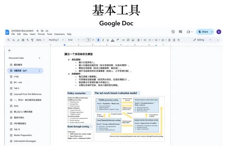
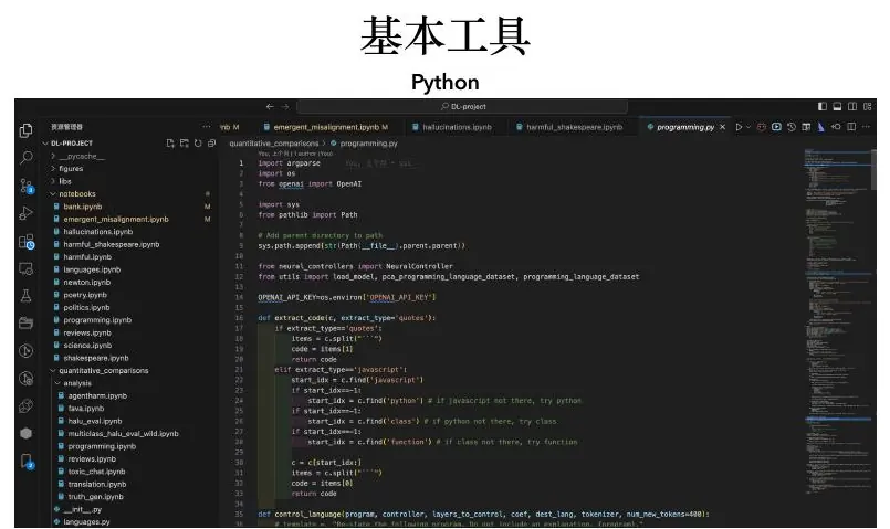
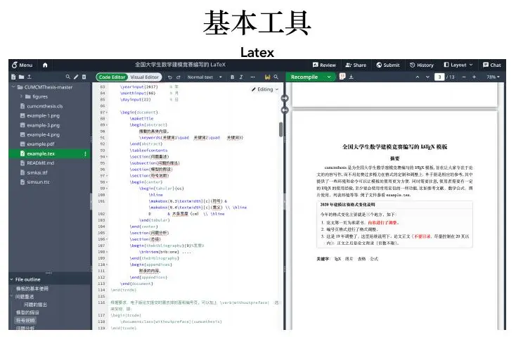
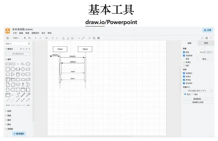
The course toolbox is a pipeline, not a list of brands. Use a shared knowledge base for task ownership; a collaborative document for live writing; Python for data, simulation, and optimization; LaTeX for the final mathematical document; draw.io or PowerPoint for diagrams; and an LLM only as an assistant whose claims and code are checked.

Let us organize the tools around one ordinary team meeting. Three students sit down with a modeling question, some data, and a deadline. One person writes the question and its subproblems in Notion or another shared notebook. The point is not the brand: it is that everyone can see the same current problem map, who owns each task, what data are missing, and which assumption has not yet been tested. If the question map lives only in one person’s head, the other two can spend a day solving incompatible versions of the problem.

Open a shared Google Doc or equivalent writing space early, even if its first version is ugly. Put in the working title, a two-sentence problem restatement, a variable table, and blank spaces for results. Why write before the math is finished? Because writing forces you to discover unanswered questions. If a paragraph says “our model predicts the best schedule” but you cannot yet say what counts as best, your objective is not fully specified. The document should track the logic of the work, not just receive it on the last night.

Use Python when the problem needs repeatable calculations: cleaning a CSV, implementing the basin recurrence, simulating customer arrivals, drawing plots, or running an optimizer. Start with a tiny test that has an answer you can calculate by hand. For our basin, the first plate should leave the water nearand the new temperature should lie strictly between the initial plate and water temperatures. If Python reports, the code failed a physical check. A script that reads raw data and produces the paper’s tables is more useful than a notebook full of manually copied intermediate numbers.

Use LaTeX or Overleaf to compose a long technical report with equations, references, and figures whose numbering stays consistent. The slide asks teams to download the current official contest template and upload it to Overleaf. That is a sensible practice task: compile a small document now, before the contest clock starts, and confirm that every teammate knows how to change a section, add a figure, and resolve a compile error. Do not wait until the last night to discover that your mathematical symbols render incorrectly.

Use draw.io or PowerPoint for a clear dependency diagram when the model has several modules. Draw arrows from raw arrival timestamps to the demand forecast, from that forecast to the staffing simulation, and from simulated waits to the recommendation. Write the units or meaning of what travels along every arrow. A nice-looking box diagram with arrows that do not name outputs is decoration; a rough diagram that exposes a missing input is useful.

Finally, you may ask ChatGPT or DeepSeek to help brainstorm a baseline, explain unfamiliar mathematics, or draft test code. Treat the output as a suggestion, not as an observation, citation, proof, or validated implementation. If it offers a basin model, check its units and whether it confuses heat capacity with temperature. If it offers a theorem for the two-day journey, check the endpoints and continuity. If it offers a source, open the actual source and make sure it supports the precise claim. The team—not the assistant—owns the result.

Here is a concrete handoff ritual that saves beginners a lot of pain. At the end of a work block, each teammate leaves three things in the shared space: what I produced, what I checked, and what the next person needs. “I made a graph” is too vague. “I generated the observed-versus-predicted arrival plot from arrivals.csv, verified that time is in local minutes, and the next step is to inspect the noon residual spike” is actionable. The same discipline scales from a two-hour classroom exercise to a three-day competition.

Python is the executable layer: every result should be reproducible from raw data.

LaTeX keeps notation, figures, tables, and references consistent.

Architecture diagrams should expose model modules and data flow.

AI can accelerate searching and drafting, but not supply evidence or responsibility.

The weekly loop is read, reproduce, generalize, and document.

A visual task graph makes dependencies and bottlenecks explicit.

We have discussed documents, code, figures, and diagrams, but it is easy to mistake a polished deliverable for understanding. So let us return to the yellow-light puzzle and hear how a modeling conversation might actually unfold at a whiteboard: questions first, physical stages second, equation third, and a challenged recommendation last.

A live modeling conversation: the yellow light

Let us model one example exactly as it might unfold in class.

Student: “Can we just look up the legal yellow-light duration?”

Instructor: We can look it up, but that answers a regulatory question, not the modeling question. We want to understand which physical quantities should determine the duration and whether the published value is reasonable for this intersection. For an actual intersection design, comply with the current applicable signal-timing rules; this exercise is about understanding the physical ingredients.

Student: “Then the variable is the yellow-light time?”

Exactly. Call it. Now ask what a driver must do after the light changes. During the perception-reaction interval, the car continues approximately at speed. That covers distance. After braking begins, a constant-deceleration baseline gives braking distance. A driver standing at the boundary of the comfortable-stopping region ismetres from the stop line. If that driver continues at speed, a simple requirement for reaching the line during yellow is

Dividing bygives

Before substituting numbers, check dimensions. Every term on the right must be measured in seconds. That one check catches the common mistake of mixing kilometers per hour with meters per second. It also reveals what the formula is saying: reaction adds a fixed time, and weaker braking or higher speed enlarges the no-comfortable-stop region. Crossing the intersection itself is a separate clearance question; it requires distance divided by speed and may motivate an all-red interval. We should not conceal the difference between getting to the line and clearing the conflict zone inside one ambiguous.

Now challenge the baseline. A downhill grade reduces effective deceleration; wet pavement lowers available friction; drivers have a distribution of reaction times; approaching vehicles do not all travel at exactly the design speed. We do not have to add everything at once. First compute a transparent nominal value. Then evaluate conservative quantiles or scenarios and report how much each assumption changes.

The conclusion should sound like this: “For the declared design speed, reaction-time percentile, effective braking rate, and clearance distance, the model requires at least ___ seconds. Wet-road and downhill scenarios increase the requirement to ___; therefore we recommend ___ with a stated safety margin.” It should not sound like this: “MATLAB outputs 4.31.” The first sentence is a decision supported by a model. The second is an unexplained number.

Here is your final thought experiment: if speed doubles, which term doubles, which term stays fixed, and which term halves? Answering that without recomputing is evidence that you understand the model’s structure.

The whiteboard conversation is the final example for today. We have moved from relationships in a commuter’s trip to continuity on a mountain path, energy accounting in a basin, and a safety threshold at a traffic signal. The same questions kept returning: what changes, what stays fixed, and what observation would make the answer unreliable? The course’s first practical assignment now asks us to recognize those questions in someone else’s completed paper, not to memorize a schedule for this chapter.

Your first week’s work: read, reproduce, generalize

The slide deck ends with a practical assignment, and I want to tell you how to do it if this is your first encounter with modeling. Start by reading several strong papers from one year’s official competition archive. Do not begin by trying to understand every line of algebra. On the first pass, ask: What real problem did the team answer? What were the three or four major steps? Which figure convinced me that the steps worked? What limitation did the authors admit? Write one sentence per answer. If you cannot answer the real-problem question, the paper’s mathematics is not yet attached to its purpose in your head.

On the second pass, trace one claim backwards. Suppose the abstract says “our proposed staffing policy reduces the mean wait by 18%.” Find the table or figure containing that result. Find the baseline used for comparison. Find the data, simulation, or field measurement that generated both waits. Ask whether both methods were tested on the same period and conditions. If one was tested on quiet mornings and the other on a holiday rush, the 18% comparison would not mean what the abstract suggests. This backwards-reading habit gives you a way to understand a technical paper without already knowing all its methods.

The course asks you to excerpt good passages and explain why they work. Do more than copy a sentence that sounds polished. Annotate its job: Did it restate the decision? Motivate an assumption? Interpret a table? Limit a claim? For example, “The policy remains feasible when arrivals increase by 20%” is useful only if the paper shows a stressed scenario and tells us what “feasible” means. A pretty sentence without attached evidence is not a model explanation. A plain sentence with a reproducible comparison can be excellent writing.

Next, reproduce three visualizations that taught you something. Choose figures with different purposes: perhaps a time-series plot for change, a map for geography, and a baseline-versus-model comparison for evidence. If the original data are unavailable, construct a small illustrative dataset and say clearly that it is illustrative rather than pretending you reproduced the exact paper. Label axes and units; explain why a line, a map, or a bar chart matches its question. When you recreate a figure, you discover how much reasoning hides in axis choice, grouping, and caption. The assignment is therefore about understanding the claim, not merely imitating colors.

The slides also ask you to reproduce the strongest paper you read. That can sound intimidating. Reproduce one small result first: a data summary, a simple baseline, or a hand-checkable intermediate calculation. Write down the inputs and expected output before running any code. If your result disagrees, distinguish missing data, undocumented preprocessing, different random seeds, and your own bug. Only then attempt a larger part of the pipeline. Reproduction is not a contest to copy the largest formula; it is a method for learning which steps in a modeling argument are actually doing work.

For “generalization,” revise an assumption in the reproduced model. If a commuter model treats all travel times as independent, ask what happens on rainy days when delays cluster. If a queue model uses one arrival rate all afternoon, ask what changes when lunchtime peaks. If a plate model assumes a heater is off, ask whether including measured energy input changes its recommendation. Make a prediction before modifying the code. Write down what moved, what stayed roughly the same, and what that teaches you about the boundary of the model.

The remaining assignment is operational: let everyone on the team become familiar with the shared notebook, document editor, Python environment, LaTeX, and diagramming tool; find legitimate materials and divide the reading; download the current official LaTeX template and make it compile in Overleaf. Think of these as rehearsal, not administrative busywork. If you know how to share a figure, rerun a script, find a source, and repair a broken equation before a timed competition, you spend the competition answering the actual question rather than fighting the tooling.

Here is a feasible calendar if you have a week. On day one, each person scans two papers and posts a one-page summary. On day two, discuss which claims are well evidenced and select one paper to reproduce. Days three and four go to one baseline and three figures, with each figure attached to a written claim. On day five, change one assumption and check the sensitivity. On day six, compile a short report in the official template. On day seven, teach the whole pipeline to another teammate in five minutes. If nobody can explain the evidence path orally, revise the report before calling it done.

Do not worry if your first attempt looks small. A defensible one-page result that answers a real question, shows a baseline, and explains a measured limitation is already a modeling achievement. Every later lecture will give you additional mathematical machinery. This first lecture gives you the habits that make that machinery trustworthy.

After practicing with published papers and the course tools, we should check whether the modeling pattern transfers beyond the slide examples. The library question below has different people and constraints but the same need for a precise decision, changing state, simple baseline, and evidence. Try it before moving to the next lecture.

A final conversation before the next lesson

I want to make sure you can use these ideas in a new situation rather than merely recognizing my examples. Imagine a library wants to reduce the number of students turned away from study rooms during exam week. Its first request is “build the best model of room usage.” Stop and ask the librarian three questions. What decision can be changed—hours, bookings, room assignments, or the number of available rooms? What outcome matters—turn-aways, average wait, student satisfaction, or unused room-hours? When is the decision made, and what data are available then? Until those answers are clear, “best model” is not a well-defined target.

Suppose the answer is: “Tomorrow morning we must decide whether to extend three rooms’ opening hours by two hours; we want fewer turn-aways, but staff time is limited to six additional room-hours.” We can now draw a boundary around arrivals, bookings, rooms, and staffing. Letbe the extra hours assigned to room. The hard rule ishours, with eachwithin the room’s permitted extension. A count of students waiting at each hour is a changing state. Historical arrival times are data. The phrase “fewer turn-aways” suggests a measurable objective. You can see a model beginning to form without choosing an optimizer yet.

Begin with a tiny baseline. If each extended room can serve one additional two-hour booking, three two-hour extensions might serve three additional groups. This is a rough upper bound only if each group’s booking takes the full interval and demand actually exists. If historical data show no one requests room three after closing, adding hours there would not help. If twenty students arrive all at once and rooms are booked in one-hour slots, our two-hour-booking assumption could misrepresent capacity. Those observations tell us which extension is worth studying: different booking lengths, hourly arrival peaks, or a better scheduling rule.

How would you test the recommendation? Use last week’s or last semester’s exam-period bookings to simulate what the proposed extension would have done, while being honest that demand can respond to added availability. Compare the same days under the existing schedule and the proposed one; report turn-aways and unused room-hours. Stress the result if arrivals rise during finals. If extending rooms one and two works on the data but fails whenever attendance is slightly higher, tell the librarian so. An actionable answer might be “extend rooms one and two first, monitor the hourly turn-away count, and revisit the assignment after one week.” That is a more modest, more useful conclusion than “our model achieves optimum efficiency.”

Can you now say how the library and the hot-water basin are alike? Both began as vague requests; both required choosing a quantity that changes—waiting students or water temperature; both had a stopping or success threshold; and both needed a test that could overturn a recommendation. Can you also say how they differ? A plate cannot choose not to enter the basin, but students may change booking behavior when rooms become available. Physical conservation gives us a strong starting mechanism in one case; human behavior may require more careful observation in the other. Learning modeling means recognizing both the transferable structure and the limits of that analogy.