Mathematical Modeling 4 - Assumptions and Architecture

The abstract gives the reader the destination. The body must show the road. Imagine a robot that reports positions from two sensors whose clocks disagree. One sensor is also noisy and may be shifted by a systematic bias. If the final path looks smooth, how would you know whether it is correct? Before fitting anything, we need a map of what each sensor reports, when it reports, which coordinate system it uses, and what each model module will pass to the next.

This lesson is about the architecture of an argument as much as the architecture of software. We will move from a precise problem restatement to assumptions attached to their equations, a notation table, a dependency graph, and a full robot-localization case. Do not worry if Kalman filters are new to you; first follow the information flowing through the system. Only after the story is clear will the equations have something real to describe.

The main body becomes clear when the architecture is clear. Before derivations, decide what each submodel receives, produces, and passes to the next stage.

Problem restatement versus analysis

A restatement translates the prompt into precise tasks without copying it. Problem analysis explains why those tasks are difficult and how they connect.

For each subproblem record:

• target quantity or decision;
• available data;
• constraints and uncertainty;
• chosen mathematical representation;
• output passed downstream;
• validation evidence.

A concise dependency map is often more useful than several pages of prose. For example:

This prevents a later optimization model from silently using information that an earlier stage never estimated.

Restatement is not a copy of the prompt

Suppose the original task says: “Two independent positioning systems observe a robot. Their startup times may differ. Some attachments contain noise and bias. Provide a high-frequency path and use it to schedule tasks.” You could paste that wording into a report under “Problem Restatement,” but then the reader has learned nothing new. Instead, make the deliverables explicit. For the idealized attachment, estimate the relative clock offset and produce 10-Hz positions. For the noisy attachment, estimate clock and fixed spatial offsets before fusion. For field measurements, test whether a fixed spatial offset is justified. Finally, use the reconstructed path to generate feasible windows and schedule as many tasks as permitted. Each sentence now names an output that can be checked.

Problem analysis goes one level deeper. Why is a clock offset hard to estimate? The systems do not sample at the same instants, so direct row-by-row subtraction is meaningless. Why can spatial bias be confused with time shift? When a robot travels steadily in one direction, moving a path along time can look like moving it along that direction in space. Why is task scheduling dependent on localization? A task may be feasible only while the robot is near a target and moving slowly enough. A timing or position error can therefore alter candidate windows. These explanations belong in analysis because they motivate the model choices and the dependency order.

Try the same distinction on the coastal-shelter case below. Restatement: choose shelters, route residents, and allocate supplies under several storm scenarios. Analysis: storm depth changes road availability; road availability changes reachable shelters; congestion changes travel time; all three alter the facility decision. A short restatement followed by an arrow chain is more helpful than a page of synonyms for “storm” and “evacuation.”

How would you know if you missed a subproblem? Make a table with one row per requested output. Include the target, input data, constraints, uncertainty, model, result, and validation. If a row’s output is never consumed or reported, ask whether it is an unnecessary calculation. If a required output has no row, your architecture is incomplete. In the robot case, “fixed-bias decision on field data” is a required output even when the decision is not to correct. Do not delete that row just because the result is negative.

Take a moment to trace one wrong architecture. If scheduling reads the raw, asynchronous source-2 coordinates directly while the abstract says it uses a fused 10-Hz path, the optimization can appear successful but be based on a different physical trajectory. The restatement says one thing, the analysis diagram says another, and the code does a third. Write down the exact table or vector flowing from fusion to scheduling so a teammate can detect that mismatch before it becomes a polished but invalid result.

Restating a problem says what we want to answer. The next risk is hiding model choices in one grand list at the front. We will attach each assumption to the particular sensor, equation, or decision that uses it, so the reader can see what breaks when it fails.

Make assumptions local

Tie each assumption to the model it supports. “Measurement noise is zero-mean Gaussian” belongs with a state estimator; “tasks cannot overlap” belongs with scheduling constraints. Local assumptions make sensitivity testing and revision easier.

Separate assumptions from observed facts. If a prompt gives daily capacity, it is a parameter. If the model assumes daily capacity remains constant next month, that is an assumption.

Let us attach assumptions to the robot rather than listing them in a ceremonial paragraph. The first alignment model treats the two records as observations of the same moving robot in the same coordinate frame. If one system reports metres in a local east–north frame and another reports latitude–longitude, neither a time shift nor a spatial bias will repair the mismatch. Check units and coordinate definitions first. If the prompt explicitly specifies a shared planar coordinate system, that is a given condition; if we infer one, it is a modeling assumption to verify.

The clock model assumes a constant offset. In words, source 2’s clock may start later, but it does not steadily drift relative to source 1 during the observed interval. A quick test is to align the first part of the path and the last part separately. If the estimated shift changes systematically, a single offset may be inadequate. An extension could use an affine map, wheredescribes drift. Do not addjust because it is mathematically available; add it when residual lag over time justifies it and when the data identify it.

The second attachment allows fixed spatial bias: one device consistently displaces positions by the same two-dimensional vector. Its reason might be a calibration error or coordinate-origin difference. Its test is whether aligned residuals have a stable mean across path segments. If residual direction rotates with the robot or changes by location, a single fixed vector is not the right explanation. A constant correction would then remove one region’s error while creating another’s.

The filter assumes the robot behaves approximately as if acceleration is constant over a short interval, hereseconds. That does not mean acceleration is physically constant for the whole trip. The state-update model needs a local approximation; process noise represents deviations such as jerks and turns. Inspect innovations, the difference between an incoming measurement and the filter’s predicted measurement. If innovations show a repeated turn-related pattern or are strongly correlated across time, the motion assumption or noise covariance may need revision.

The schedule assumes each candidate task has a preparation window and that device-resource rules are enforced. The supplied report treats shooting and photography devices as independent resources and checks non-overlap inside each class; it also adds an angle rule for repeat photography. These are operational assumptions or prompt rules, depending on what the task specifies. If the two devices share battery or operator time in reality, independent scheduling could overcommit the robot. Test that dependency before applying the plan outside the modeled setting.

For each assumption, write four things beside it: why it is plausible, which equation it enables, what its failure would do to the final decision, and what observation would expose that failure. “Constant clock offset” enables a one-parameter alignment; its failure can shift task windows; segment-wise lag is a test. “Fixed bias” enables a two-coordinate correction; its failure can bend the fused path; segment-wise residual means are a test. The list becomes useful when every row has such a consequence and check.

Here is a subtle beginner trap: an observed number is not an assumption simply because it is entered into a model. The measured timestamps are data. Their correctness and synchronization conventions may be assumptions. A 10-Hz output requirement is a specification; the claim that a 10-Hz interpolated path captures all relevant motion is an assumption. Distinguishing these categories prevents a report from pretending that provided conditions were “validated” or that assumed conditions were “given by the problem.”

Design notation as an interface

Notation should reduce cognitive load. Establish consistent rules:

• sets use calligraphic capitals, such as;
• parameters use known data, such as demand;
• decision variables are visibly distinct, such as;
• estimated parameters carry hats, such as;
• vectors and matrices use a consistent bold convention.

Define indices and units. Avoid reusingfor both time and a threshold. A symbol table should contain only symbols that recur; a variable used once is better defined beside its equation.

Notation is not a test of how many Greek letters you know. It is an agreement among the person writing the model, the person implementing it, and the person checking it. Imagine that one teammate writesfor the shift added to source-2 timestamps, while another writesfor the shift subtracted from them. Both can produce plausible curves and opposite reported signs. Decide the convention in a sentence: “Source 2’s printed clock is ahead of the common physical clock by, so physical time is.” Then the comparisonversushas a consistent meaning. If a teammate chooses the opposite convention, they must also reverse the sign of the reported offset.

Units make the agreement even more concrete. Robot positionis in metres; velocityis metres per second; accelerationis metres per second squared; a clock offsetis in seconds; a spatial biasis in metres. A residualis a position difference in metres. Its squared norm has units of square metres. If you accidentally compare a timestamp in milliseconds with one in seconds, the alignment search may run but its result will be nonsense. A unit column beside each recurring symbol is a cheap guard against this mistake.

Indices also matter. Letindex source-1 samples,source-2 samples, andpoints on the common 10-Hz grid. Those sets have different sizes because sensors sample at different rates. Writingpretends that rowfrom both files refers to the same physical moment. The index notation itself warns you that the pairing is invalid. An interpolant or common-time projection is needed before subtraction.

Be consistent about the six-state vector. The supplied robot report uses. With that order, theone-axis transition matrix can be placed twice on a block diagonal. If you rearrange it tobut keep the same block-diagonal matrix, you will update the wrong physical quantities. A symbol table should state the order explicitly, and code tests should verify that one metre-per-second ofchangesbymetre over a-second step when acceleration is zero.

Now compare state, parameter, and decision notation. A filtered robot positionis an estimated state. Clock offsetand biasare estimated calibration parameters. A binary task variableis a schedule decision for candidate. Writing them all aswith different subscripts would be legal mathematics but costly for a beginner’s memory. Distinct names help you see which quantity changes because of a new sensor reading and which changes because an optimizer chooses a different plan.

Keep the symbol table lean. Define a long-lived variable once and use the same letter across the analysis, equations, code, tables, and figures. Define a one-off quantity right beside the equation where it appears. Before submission, search for every symbol in the table and check that it appears in the body; search for every recurring symbol in equations and check that it has a definition. An unused table row is clutter; an undefined recurring symbol forces readers to guess the model’s interface.

Connect data to equations

Every parameter in an optimization or simulation must have a source. Build a parameter lineage table:

Parameter	Meaning	Unit	Source or estimator
	demand in period	units/day	cleaned observations or forecast
	assignment cost	dollars	distance and labor model
	scenario probability	dimensionless	empirical frequency or assumption

This table catches inconsistent units and unexplained constants before they enter code.

Look atin the table. “Assignment cost” could mean money, travel distance, travel time, or a weighted score. You cannot give it a dollar unit merely because the objective is called cost. Ifis distance in kilometres and the optimizer minimizes, the objective has units of person-kilometres whencounts people. If you mean monetary transport cost, multiply distance by a specified cost per person-kilometre, or model vehicles and trips more realistically. A lineage row should show that conversion instead of presenting a mysterious fixed coefficient.

For storm scenarios,may be an estimated probability from historical events or a deliberate modeling weight. If it is a probability, requireand. If scenarios were invented to stress a plan, do not label their weights as real-world probabilities without calibration. The optimizer can still evaluate them, but the resulting “expected” score has a different interpretation. A dimensionless number can be mathematically well formed and empirically unsupported; lineage checks both properties.

The robot has similar parameters. Measurement covarianceshould be connected to sensor quality, repeated measurements, or a stated calibration procedure. Process covarianceshould be connected to motion-model mismatch, not chosen solely until a final plot looks smooth. Preparation timeshould come from the task rule or a measured device requirement, with seconds as its unit. Target coordinates need a source and the same coordinate frame as the robot path. If one target location is in centimetres while positions are in metres, a distance test can reject every task or accept absurd ones without any solver error.

Some parameters are estimated from the same data that later produce a result. That is allowed, but it means the result is conditional on the estimation procedure. Ifandwere fitted using the entire field path and the same path was then used to report an “independent” alignment score, that score is in-sample. A held-out segment or separate calibration run provides stronger evidence. The lineage table can say not just “estimated from trajectories,” but which segment was used for fitting and which for checking.

One useful habit is to follow a final number backwards before submission. If the shelter plan costs, find the cost coefficient for each opened shelter, its data source, and the exact sum in the objective. If the robot’s selected task count changes when target coordinates are corrected, find which file version produced the old count. A model may be mathematically elegant yet unusable if its parameters cannot be traced to observations, prompt conditions, or explicitly labeled assumptions.

Use model layers

A strong architecture often has four layers:

1. data layer: cleaning, alignment, interpolation, feature construction;
2. descriptive layer: exploratory patterns and parameter estimation;
3. decision layer: optimization, simulation, or policy selection;
4. evidence layer: residuals, held-out tests, sensitivity, and alternatives.

Not every problem needs all four, but the separation prevents data preprocessing from being mistaken for a model and prevents solver output from being mistaken for validation.

Use the coastal city to see why layers matter. The data layer reads elevation, roads, shelter locations, and neighborhood counts, fixes coordinate and unit mismatches, and marks missing values. The descriptive layer estimates which cells may flood and how many residents are likely to need evacuation under each scenario. The decision layer chooses shelter openings, routes, and supplies subject to capacity and cost. The evidence layer asks whether the selected plan actually gets people to safety under congested or unexpectedly severe conditions. If a flood map is treated as a final shelter plan, a whole decision step is missing. If a solver’s selected shelters are called “validated” without testing travel and overflow, the evidence layer is missing.

For the robot, cleaning timestamps and checking coordinate frames belong in the data layer. Estimating the clock shift, spatial bias candidate, and filtered path belongs in the state-estimation or descriptive layer. Generating feasible tasks and selecting a schedule belongs in the decision layer. Objective curves, withheld interpolation points, residual plots, BIC comparison, path error, and final constraint checks belong in the evidence layer—although some evidence checks should occur between stages, not only at the end. This separation lets a reader see which numbers were observed, which were estimated, and which were chosen.

Do not force every activity into a single box. Interpolation is a data transformation, but its choice also requires evidence because it influences alignment. Bias diagnosis compares descriptive models and affects a decision about correction. A model architecture is a teaching map, not a prison for methods. Its value is that no stage can silently borrow an output from the future or present an untested transformation as fact.

Parameter lineage is the same idea at a smaller scale. Suppose a shelter travel-time matrixis used by an optimizer. Which roads, speeds, storm closures, and congestion assumptions produced it? The body should identify that source. Suppose the robot schedule uses speedand acceleration. Did they come from the filtered state, a smoothed offline state, or a finite difference of raw positions? If the task count depends on that choice, the data source must be stated. A final result inherits every upstream estimation choice, whether or not the optimizer’s own code is perfect.

Draw one arrow and ask a teammate to read it. “Hazard model to location model” is too broad. “Road-open indicator, dimensionless, plus travel-time matrixin minutes” is an implementable contract. “Fusion to schedule” is too broad. “10-Hz state rows containingin seconds,in metres,in metres per second, and uncertainty” tells the next module what it receives. The arrow label helps a human reason and helps code validate shapes and units automatically.

You can also trace a number backwards. If the final shelter result says 95% arrive in 45 minutes, find the simulation events that determined arrival times, the assignments that determined routes, the road-open states that determined which routes existed, and the raw elevations or flood observations that determined those states. A missing link is not merely a documentation flaw; it may be an unexamined assumption that could change the recommendation. The four layers make that backward search manageable.

Plan before coding

Write a one-page model specification containing the objective, state or decision variables, constraints, data inputs, expected outputs, and tests. Then construct a minimal synthetic case whose answer is known. A scheduling model should solve a two-task example by inspection before it is trusted on 10,000 tasks.

The architecture is successful when another teammate can implement one stage without guessing what the previous stage meant.

What belongs on that one-page specification? For robot alignment, write the input files and their timestamp and coordinate conventions, the sign convention for, the overlap rule, the alignment objective, the expected synchronized output table, and two tests: a known-shift toy path and a withheld-time comparison. For the filter, write the exact state order,-second update interval, position-only observation map, sources forand, and a constant-speed toy check. For scheduling, write the candidate-window generator, resource non-overlap, angle and preparation rules, objective, and a two-task hand case. That page is more useful than a folder full of code with no shared meaning.

Suppose two photography candidates refer to the same target and their camera angles differ by, while the rule requires at least. Your hand case should reject selecting both. Change the second angle so the difference isand let them occupy non-overlapping windows; both may be feasible. If the code gives the same answer in both cases, it probably forgot the angle constraint. A unit test anchored in the prompt’s rule gives you far more confidence than a large solver run that returns a plausible-looking task count.

For clock alignment, generate the three-point source records with known-second shift described above. The code should recover the declared sign and synchronize the output timestamps. For the filter, feed a noiseless robot moving at 2 m/s with zero acceleration and check that its predicted position advances by 0.2 m over one grid step. For bias diagnosis, give it a zero-bias noisy toy and ensure it does not always invent a fixed correction merely because the residual sample mean is nonzero. These tests isolate different interfaces; a final trajectory plot cannot tell you which one broke.

When you hand work to a teammate, include a small schema. A synchronized observation table might have columns common_time_s, source_id, x_m, y_m, and measurement_covariance. A task-candidate table might have target_id, start_s, end_s, task_type, angle_deg, and constraint_passed. Names are not the mathematical model, but explicit units and meanings prevent accidental confusion. If the output shape changes, update the schema and the diagram together.

Only after the specification and tiny checks agree should the team scale to thousands of samples or candidate tasks. This order can feel slower during the first hour, but it saves hours of debugging a discrepancy that arose from a symbol or unit mismatch. Planning is not avoiding code; it is making the code answer the same question the paper claims to answer.

I would run a fifteen-minute architecture meeting before the team splits up. The person handling sensor data reads the timestamp and coordinate conventions aloud and shows one row from each file. The person handling fusion reads the state order and expected synchronized input schema aloud. The person handling scheduling states which path table they will consume and which task constraints they will implement. The writer listens for words that mean different things to different people—“offset,” “bias,” “feasible,” “time window,” “optimal”—and records a one-sentence shared definition for each.

Suppose the data teammate says, “Source 2 starts fifty seconds later,” but the fusion teammate’smeans “source 2’s printed clock is ahead by fifty seconds.” Are these the same statement? Not necessarily; later physical startup and an ahead-running clock are different descriptions. Use the known-shift toy path and one real overlapping segment to settle the convention. Suppose the scheduling teammate says “task at time 10.0 is feasible,” but the prompt requires ten seconds of preparation beforehand. Ask whether the entire intervalwas checked. A short meeting can find these semantic gaps before they spread through code and prose.

Put a small status card beside each module: input received, output produced, sanity check passed, evidence still missing. For alignment, a known-offset toy passing is an implementation check; a real objective curve and withheld comparison are evidence. For fusion, a constant-motion toy passing is an implementation check; a residual plot and reference error are evidence. For scheduling, a two-task conflict passing is an implementation check; a final selected interval table and stressed feasibility are evidence. Do not call a module “done” merely because it exported a file.

If a later test fails, return to the card for the specific interface instead of rewriting the whole model at once. A changed clock estimate should update synchronized observations, fusion, task candidates, and reported counts in that order. A changed target coordinate should update candidate windows and schedule but need not refit sensor alignment. The dependency graph tells us what must be rerun. This is practical long-term maintenance as well as sound mathematical communication.

At the end of the meeting, everyone should be able to answer the same question: “Which file and mathematical object would we hand to the next person?” If three people give three answers, the architecture is not yet ready. Fixing that disagreement is real modeling work, even though it produces no glamorous plot.

Do not mistake the diagram itself for the architecture. The architecture also lives in variable definitions, input schemas, a test dataset, and the order in which results are refreshed. A picture can show where an arrow goes; a schema says what crosses it; an assumption explains why that transfer is legitimate; a test says how we would notice if it failed. When all four agree, the main body reads like a connected explanation rather than a sequence of unrelated chapters. That connection is what allows a skeptical reader to move from the abstract’s headline number back to its original measurement without guessing.

If this lesson felt like several topics—restatement, assumptions, notation, data lineage, alignment, filtering, and scheduling—return to the single robot question at the top. Each topic repaired a different possible break in the same path from raw sensors to actionable tasks. That is the thread to remember when you face a new prompt: do not ask which chapter heading to imitate; ask where information could be lost, distorted, or used before it exists.

Architect a multi-part problem

Consider a coastal city deciding where to place emergency shelters, how to route residents, and how many supplies to pre-position under uncertain storm intensity. The prompt appears to contain three independent questions, but a good architecture exposes their interfaces.

Let us pose the question as a city official would. Three neighborhoods may need evacuation tonight. A severe storm might flood a bridge, and not every shelter can hold everyone. The official can choose shelters before the exact storm is known, but drivers may choose routes after road closures are announced. “Where should shelters open?” and “How do residents get there?” are therefore linked but not identical decisions. If the city treats them as three unrelated spreadsheet tabs—shelter sites, routes, supplies—it might choose a cheap shelter that residents cannot reach in the severe scenario.

For a first hand-checkable instance, suppose neighborhoodshave 100, 80, and 60 evacuees, respectively, and shelterscan hold 150 and 120. The total need is 240, the total nominal capacity 270. That surplus of 30 looks comforting, but ask whether routes connect the right people to the right beds. If a flooded bridge blocksfrom, all 60 frommust reach. The remaining 60 beds atcan serve others;can hold up to 150. One feasible assignment is 100 fromand 50 fromto, then 30 fromand 60 fromto. Check sums aloud:sends;receives 150;receives 90. All 240 people are assigned without exceeding either capacity.

Now change one road assumption. What if the route fromtois also flooded? Then our assignment fails even though the city still has 270 beds. Ifcan reach only,andtogether need 180 beds there, more than its 150 capacity. The city may need another site, a temporary bridge route, or a transport plan that changes which roads are feasible. A numerical total-capacity check cannot detect a network accessibility failure. That is why the hazard map must feed the road graph before facility allocation is declared feasible.

The example also shows the supply interface. If one resident needs three litres of drinking water per day, shelterin our first assignment needs at leastlitres per day;needs. If the plan is for two days, double these baseline volumes and add a margin for uncertainty and staff. Supply allocation should consume the chosen resident assignment, not guess independently from shelter capacity. Sending two days of water for 120 people towhen only 90 are assigned may be reasonable as a reserve, but the model should label it as a deliberate safety margin, not an unnoticed mismatch.

We can now draw the module arrows with names. A storm scenario produces flooded cells and a binary road-open table. That table and an evacuation-demand table feed a network model, which produces reachability and travel-time entries for each neighborhood–shelter pair. The facility model uses those entries, shelter capacities, and costs to choose open sites and allocations. The chosen allocation produces supply requirements. A simulation uses the plan, uncertain arrival times, and road capacities to estimate congestion and overflow. These arrows are the architecture; without named information on them, “four models” is just four boxes in a picture.

Build a dependency graph

The hazard model estimates flooding by location and scenario. Its output determines which roads are available and how many residents require evacuation. The network model estimates travel time and accessibility. Those quantities enter a facility-location model that selects shelters and allocations. A final simulation tests congestion, shelter overflow, and supply exhaustion.

Write every arrow as data: “hazard modelroad-open indicator,” not merely “Model 1 supports Model 2.” If an arrow has no named output, the modules are not yet connected.

Define states, decisions, and parameters

For scenario, letindicate whether road edgeis usable andbe evacuees at neighborhood. Letindicate whether shelteris opened andthe scenario-dependent number sent fromto. The distinction matters:is a here-and-now decision, whilemay adapt after the storm scenario is known.

The phrase “under severe storms” must become a scenario set, probability model, or bounded uncertainty set. A verbal adjective is not a mathematical input.

Let us write the most important constraints in words before symbols. Every neighborhood’s evacuees must be assigned somewhere reachable. A shelter can receive people only if it is open. The total assigned to a shelter cannot exceed its capacity. A closed road cannot carry a route. Those are not optional properties of an objective function; they are the physical rules that define a feasible plan.

For each scenario, a demand-balance rule isif every resident must be assigned. A shelter-capacity rule is, whereis its capacity andcloses it. If road access betweenandis impossible in scenario, set the correspondingor omit that assignment edge. Check units:andcount people,counts people, andis dimensionless. It would be nonsensical to add travel time in minutes to one side of a capacity inequality in people.

Why doeslack a scenario index whilehas one? The city opens shelters before it knows which storm will occur. That is a here-and-now decision. Routing may adapt after roads and demand are observed, so allocations can be scenario-dependent recourse. If the city actually must print a fixed route plan the day before and cannot adapt,should not silently depend on; the model then needs a plan feasible across declared scenarios or an explicit contingency rule. Index choices encode what the decision-maker can know and change at each time.

Do we need scenario probabilities? If the objective minimizes expected travel time, then each scenario needs a probability or weight with a credible interpretation. If the city wants a plan that stays feasible under every severe scenario in a stated set, we can use robust constraints without pretending to know frequencies. If it cares about a 95th-percentile overflow rate, we need a chance or simulation interpretation. These approaches answer different policy questions. Saying only “under uncertainty” is not enough to choose among them.

Try a sanity test before a solver. Open both shelters in the hand-checkable example and feed the assignment with 150 atand 90 at. Does the code mark it feasible? Closeand leave 90 people assigned there. Does it mark that infeasible? Close theroad in the severe scenario. Does the assignment fail? If any answer is surprising, debug the data-to-constraint interface before running a large city network. A three-neighborhood toy is a unit test for the architecture.

Audit assumptions by module

The hazard layer may assume elevation data are accurate; the network layer may assume travel time depends on flow; the location layer may assume shelters meet a minimum safety class. Do not place all assumptions in one undifferentiated list. A local assumption is easier to test and revise. For each one, state which equation or data transformation it enables.

Specify interfaces before implementation

Create a contract for each module:

Module	Inputs	Outputs	Required checks
Hazard	elevation, storm scenario	flooded cells,	compare with historic flood maps
Network	graph,, demand	travel-time matrix	connectivity and flow conservation
Location	travel time, capacity, cost		budget, capacity, integrality
Simulation	selected plan, event distributions	delay, overflow, failures	repeated seeds and extreme scenarios

This table also defines a clean software structure. Each module can be tested using synthetic inputs before the preceding module is finished.

Trace one number end to end

Choose a final result—say, “95% of residents reach shelter within 45 minutes”—and trace it backward. Which simulation output creates it? Which routes and assignments create those trips? Which road states and storm scenarios create the network? Which raw measurements create those states? If any transition is undocumented, the result is not reproducible.

Be precise about that 95%. Does it mean 95% of all simulated residents, 95% of scenarios, or 95% of neighborhoods? Those denominators give different claims. If the simulation sends 240 residents and 228 arrive within 45 minutes,of residents in that run. If 19 of 20 scenarios meet a policy target, that is 95% of scenarios. A figure or abstract that reports “95% success” without the denominator breaks the evidence chain even if its arithmetic is correct.

For the resident-level claim, trace one late arrival. Which shelter was that person assigned to? Which route did they take? Was a bridge closed in that scenario? Which travel-time estimate and congestion rule determined their arrival clock? Then trace that road state back to flood elevation and storm-intensity assumptions. A model architecture is not fully tested when you can only reproduce the aggregate 95%; you should be able to explain an individual failure that contributed to the other 5%.

The backward trace also reveals feedback. Suppose the location model choosesbecause the network model predicts a short route. Once many residents choose, that route becomes congested, making it slower. A one-way pipeline “network travel timeshelter choice” hides this response if travel time actually depends on selected flow. You may need an iterative assignment, a joint traffic–location model, or a scenario simulation that evaluates and revises the choice. Draw the feedback arrow and say what updates on each iteration. An unlabeled circular arrow is no better than pretending congestion does not exist.

This is a common modeling boundary decision. If added traffic barely affects travel time, a fixed travel-time matrix may be a credible baseline. If the roads are near capacity, feedback may reverse which shelter is best. Test a few flow levels before choosing the complexity. The graph should make the simplification explicit: “Travel time is fixed at the measured baseline for the first model” is a statement one can challenge. “The network model feeds the location model” alone is not.

Finally, ask whether the official can actually use the proposed adaptive allocations. If routeschange after storm scenariois known, who communicates the new route and when? If the decision must be printed on evacuation signs before the storm, the scenario-dependent solution may be mathematically feasible but operationally impossible. The architecture needs an information timeline as well as a data-flow graph. A result can fail because a decision is made too late or assumes future knowledge, even when every numerical constraint is satisfied.

Practice

Take a problem with at least three subquestions. Draw a directed acyclic graph whose nodes are model modules and whose edges are named tables, vectors, or parameters. Mark each quantity as observed, estimated, assumed, decided, or simulated. The finished graph should let a teammate identify circular dependencies before any code is written.

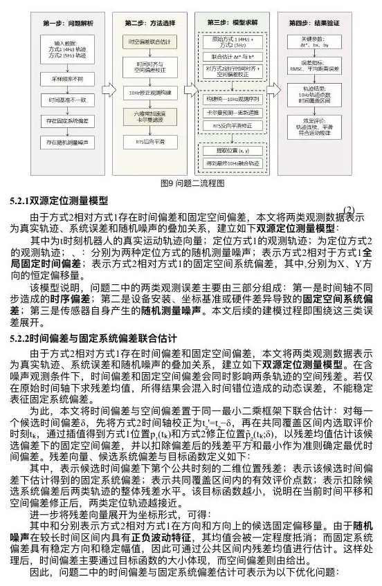
Our architecture checklist can look abstract. The robot case makes each interface concrete: two positioning systems report at different times, and a position estimate cannot be trusted until we know how their clocks, coordinates, and uncertainties connect.

Full course case: asynchronous robot localization

The writing lectures use one continuous case. A robot travels while two positioning systems record coordinates with different startup times, sampling rates, random noise, and possible fixed spatial bias. The fused 10 Hz trajectory is then used to schedule shooting and photography tasks. Estimation and decision must remain connected without being confused.

Four deliverables

1. Estimate a pure time offset from noise-free position records and reconstruct a 10 Hz path.
2. Estimate time and fixed spatial offsets under noise, then fuse observations.
3. Decide whether field data support a fixed bias before correcting it.
4. Maximize feasible tasks under range, dwell-time, device, and turning constraints.

Tasks 1–3 estimate state; task 4 consumes that state. If task 4 silently reads raw observations, the architecture is broken.

Let us walk the raw-to-decision chain with a clock. Source 1 records a positionat its own time. Source 2 records another position at its own. We first inspect each track separately: are coordinates in the same units, how often is each sampled, are there missing intervals, and do both describe roughly the same route? These are observations and data-quality checks, not yet evidence of any fixed clock shift. If the path shapes differ dramatically, forcing one global offset may be meaningless.

For the noise-free attachment, the supplied course example reports a relative startup offset ofseconds after continuous-trajectory alignment and outputs 7,004 positions at 10 Hz. A near-zero reported alignment discrepancy belongs to this idealized attachment. Do not carry its precision into the noisy case as if the second dataset had the same conditions. The second attachment reports a-second offset and a fixed spatial bias vectormetres before state fusion; its reported fused-path RMSE ismetres. The field attachment then tests a candidate fixed bias of magnitudemetres, sees only aRMS improvement and a larger BIC, and declines the correction. These numbers are from different parts of the supplied report, and keeping them in their proper modules is an architectural requirement.

The outputs passed downstream should have names and shapes. Alignment producesin seconds, possiblyin metres, and synchronized observation rows on a common clock. Filtering produces a 10-Hz table whose rows carry time, estimated position, velocity, acceleration, and uncertainty. Bias diagnosis produces a yes/no correction decision with diagnostic evidence. Candidate generation consumes the final path and target coordinates, and produces task windows that passed distance, motion, and preparation-time rules. Scheduling consumes those windows and produces selected task IDs and time intervals. A teammate who receives only “the trajectory file” should ask whether it is raw, aligned, filtered, smoothed, or bias-corrected; otherwise a small filename confusion can invalidate the schedule.

One high-level graph makes the logic easier to see: raw samplesclock and coordinate checkalignment parameterssynchronized observationsfiltered and possibly smoothed statefield-bias decisiontask candidatesselected schedule. Put validation checks beside the stages they test, not only at the last arrow. A maximum alignment error tests the first stage under its dataset; a held-out position error tests trajectory reconstruction; constraint checks test the schedule. If a final task count looks good but the fusion path is off by metres, the last-stage score is not evidence that the early stages worked.

Notation is the interface shared by alignment, fusion, diagnosis, and scheduling.

Initial plots compare sampling, path shape, and possible temporal displacement.

Aligned paths and residual panels test whether a clock shift is sufficient.

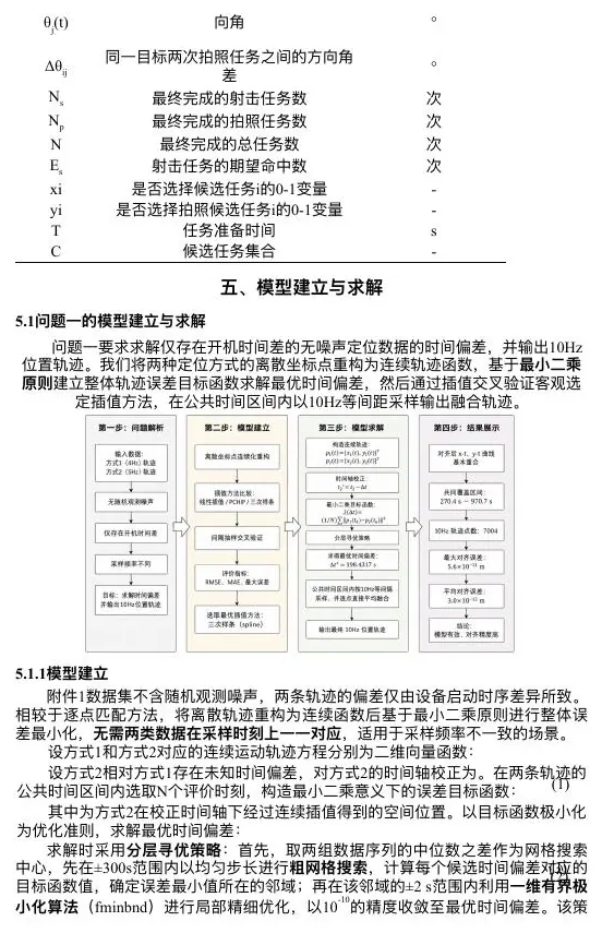
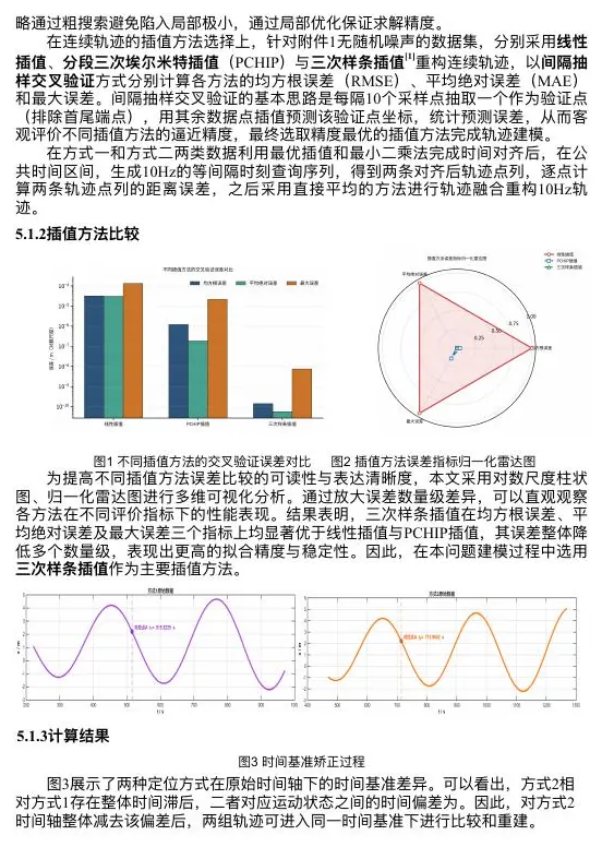
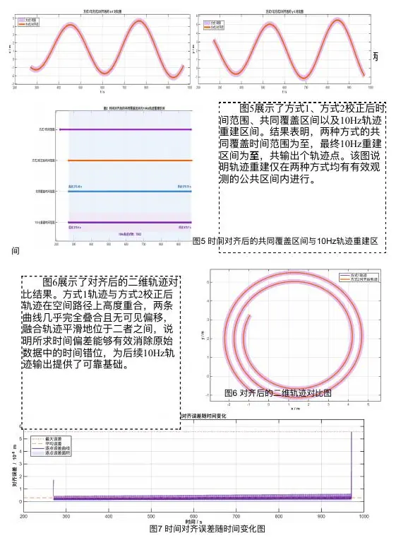
Use the three pictures as questions, not as proof by decoration. The notation table should let you find the unit and role of,, and the state vector without guessing. The initial source plots should reveal which device sampled more often, whether both follow the same route, and whether there are gaps where interpolation will be uncertain. The alignment diagnostic should show more than two curves that visually overlap: inspect its residual scale, the objective near the selected offset, and any path segment where disagreement remains. A wide screen can make a metre of error look tiny beside a kilometre-long route; use a residual panel with metres on its axis.

Now imagine the pictures disagree. The notation table says source-2 coordinates are metres, but an axis label says centimetres. The route plots look similar but the residual panel shows a steady eastward displacement after time alignment. Do not simply caption the figure “excellent alignment.” Check units and the spatial-bias hypothesis. If residuals change sign at turns, revisit the time shift or motion model. A figure can be an evidence interface only when the body explains what discrepancy would trigger which modeling revision.

Continuous-time alignment

Let source 1 provideand source 2 provide, where. Pointwise subtraction is invalid because timestamps differ. Build continuous interpolantsand. For clock offset, minimize

The overlap setmust be recomputed for every candidate; otherwise large offsets can appear good because fewer points remain. Use a coarse grid to locate a basin and bounded refinement to obtain precision. Plot: a flat or multimodal curve means the offset is weakly identified.

Interpolation is part of the observation model. Linear interpolation is conservative but nonsmooth; cubic splines are smooth but may overshoot turns. Test both on withheld timestamps. Smoothness is not evidence of accuracy.

A three-point clock example you can check yourself

Before optimizing, imagine a robot moving one metre to the right every second. Source 1 records. Source 2 watches the same motion but its printed clock is three seconds ahead: its rows are. If you compare row one with row one, the positions match, but the timestamps do not. If you compare equal printed times, there are no shared times in this tiny example. The physical agreement isfor, so the estimated offset in our declared convention isseconds.

Suppose source 2 records at timeswhile source 1 records only at. There still is no one-to-one row pairing. A continuous interpolant lets us ask what source 2 would have reported at printed time, or what source 1’s path was at physical time, under a declared interpolation rule. For constant straight-line motion, linear interpolation is exact. For a sharp turn, a cubic spline can overshoot a corner; a plot that looks smooth can be physically wrong. Hold out some measured timestamps, interpolate from the rest, and compare the interpolated positions with withheld measurements before using the interpolant inside clock alignment.

Why divide the objective by? As a candidate offset changes, the time interval where both reconstructed paths exist can shrink. If we sum residuals without accounting for the number of comparisons, a large wrong offset with only a few overlapping points may appear to have a small objective simply because it has almost no points. Dividing by count gives a mean squared disagreement, but it is not the whole solution. An offset with only two matched moments is still weakly supported. Require a minimum common duration or sample count and show overlap size alongside the objective curve.

Why search coarsely then refine? If the startup gap could be hundreds of seconds, a coarse grid can reveal where disagreement is low without spending fine resolution everywhere. A local bounded search can refine near that basin. But do not trust the first narrow minimum if the path repeats a loop. Two different shifts may line up similar route segments and create two minima. Plotover the full plausible range, inspect whether minima are distinct, and check a withheld segment. If the curve is flat, report weak identifiability rather than printing a six-decimal offset with false confidence.

Finally, the sign convention needs an implementation test. For the toy rows above, an algorithm using our formula should reportseconds, because source 2’s printed clock is ahead. If it reports, the algorithm may use an equally valid opposite convention—but then the report and correction code must say so consistently. A simple known-shift dataset lets you verify that the symbol, the objective, the synchronized output timestamps, and the sentence in the abstract all agree.

Joint temporal and spatial calibration

With constant bias,

For each, the least-squares estimate ofis the mean aligned residual. Substitution reduces a three-parameter search to one dimension:

On a nearly straight constant-speed path, a clock shift and displacement along travel can imitate each other. Turns and acceleration provide the excitation required for identification.

Let us see that ambiguity with numbers. Suppose the robot travels east at exactlymetre per second. If I move source 2’s timestamps forward by one second, its positions appear one metre farther east at a matched physical time. If instead I leave the timestamps alone and subtract a one-metre eastward spatial bias, the two paths may agree just as well. On this straight constant-speed segment, the data may not tell us which explanation is correct. A solver can still outputand; precision in its printout is not evidence that the pair is uniquely identified.

What would help? A turn. Suppose the robot moves east and then north. A time shift causes disagreements along the current direction of travel: east on the first segment, north on the second. A fixed spatial bias keeps the same east–north vector through both segments. Compare residual patterns around the turn. If one clock shift aligns both east and north motion while one fixed bias remains stable, the parameters become easier to distinguish. Accelerations and speed changes can provide similar information. This is what “excitation” means here: the motion varies enough that different parameter explanations produce visibly different predictions.

The mean-residual formula forcomes from ordinary least squares. At a fixed time shift, compute aligned differences. If we assume one constant bias vector, we choose it to minimize. The minimizer is their mean. You can confirm with a one-dimensional toy residual listmetres: their mean ismetres; subtractingleaves residualswhose squared sum is. Subtractingleaveswhose squared sum is. This explains why the vector mean is used, not merely that a formula exists.

But a mean can be distorted by outliers. If one sensor reading is corrupted, an extreme residual shifts the mean and therefore the bias estimate. Plot residuals, inspect unusual readings, and consider robust fitting or a predeclared quality rule if the attachment requires it. Do not quietly discard inconvenient points after seeing which choice improves the final RMSE. Any rejection rule should be stated and its effect checked. A good body section tells the reader how calibration parameters were estimated and how fragile they are to the data quality we actually observed.

The final joint objective searches over time shift after removing the best constant bias at each shift. This reduces the numerical search from a three-dimensionalproblem to a one-dimensional search over, withcomputed analytically. That is a practical simplification, but it does not eliminate the identifiability problem on straight motion. The objective curve and segment-wise residual checks are the evidence that the reported pair represents the data rather than one arbitrary member of a long valley of equivalent explanations.

The objective and synchronized paths should agree on one offset.

Calibration, resampling, filtering, smoothing, diagnosis, and output remain separate.

Source-wise residuals show where a shared state succeeds and fails.

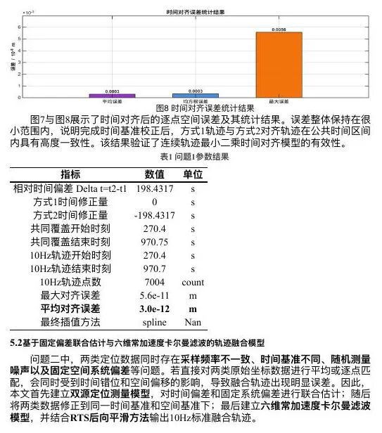
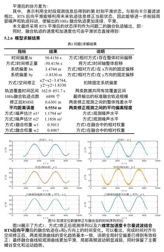
The synchronization result image should connect to the selectedand common overlap interval. The fusion architecture image should match our actual module order: calibration, resampling, filtering, smoothing, bias decision, and final path. The aligned-source comparison should let the reader see whether one sensor systematically differs from the shared state or whether errors are transient. If a method figure has a box that never appears in the equations or code, the architecture is overstating the work. If the text estimates a parameter that has no visible place in the picture, decide whether the picture needs that stage or whether the parameter is a low-level detail best explained in a caption.

Six-state constant-acceleration filter

Ats use the six-state order in the supplied report,. For one axis,

With the declared state order, the full transition is. If you instead order positions first, the same block-diagonal matrix would update the wrong components; change the matrix with the state order rather than mixing conventions.

Measurements observe position only. Prediction and update are

represents unmodeled jerk andsensor uncertainty. Estimate them from calibration or residuals. RTS smoothing is appropriate offline because future data revise past states; do not describe it as a real-time algorithm.

Read the filter as a motion story

The six numbers inare not six mysterious knobs. They say where the robot is in, how quickly it is moving in, how itsspeed is changing, and the same three facts in. At each-second step, a constant-acceleration prediction says;;. Theequations have the same form. This is the motion model behind the matrix.

Check it on a tiny instance. Ifm,m/s, and, one step predictsm. Ifm/s, the additional acceleration term ism and the nextism/s. If your code instead changesbym while, the state order or transition matrix is wrong. A two-line hand calculation can catch a matrix permutation that would be almost invisible in a smooth long trajectory.

The sensors do not directly report velocity or acceleration in this setup; they report noisy positions. The observation matrixtherefore selects theandcomponents from the state. When a new position arrives, the filter compares it with the position predicted from motion. Their difference is an innovation. If the measurement is relatively reliable, the update moves the estimated state more toward it. If the measurement is noisy, the filter relies more on its motion prediction. The Kalman gainis the mathematically computed weighting under the declared covariance model; it is not a dial that we set by visual taste.

The matricesandhave different jobs.represents uncertainty in the motion prediction—jerk, turns, or other behavior the constant-acceleration step did not explain.represents uncertainty in an arriving observation. Two devices may have differentvalues; using the same arbitrary noise level for both would ignore information about their measurement quality. Estimate plausible scales from calibration, residuals, or repeated measurements and report how path results change if those scales are wrong.

We also need a time-information distinction. A filter at timeuses observations available up to, so it can support an online estimate under the model. An RTS backward smoother runs after the full record is available and uses later observations to revise earlier states. It can make a cleaner historical path for offline analysis and scheduling on a completed trajectory. It cannot be described as what the robot knew in real time before the later observations existed. If the task schedule is for future online operation, model that information constraint explicitly.

What would reveal a failing motion model? Plot innovations over time and compare them with known turns. If they cluster at turns, constant acceleration between steps may be too crude. If innovations from both sensors move together, they may share a common disturbance, violating a simple independence assumption. If a sensor systematically reports one direction too far, revisit fixed bias rather than inflating random noise until the residual plot looks harmless. Every diagnostic suggests a different architectural repair.

The filter’s output should be a table of common-grid time, estimated state, and uncertainty, with units attached. A schedule optimizer should not need to reconstruct hidden velocity from unsynchronized raw positions if the fusion stage already estimates it. That is why we defined the output contract before diving into matrix equations: the equations produce information that the next decision stage can actually use.

The filter gives us a prediction and a residual. A residual pattern is not automatically a new physical law or a code bug; it is a clue. We will ask which measurable bias could produce it and how an independent check would distinguish that explanation from others.

Bias is a hypothesis

A nonzero residual mean can arise from noise, interpolation, transient motion, or real fixed bias. Compare no-biaswith biasusing held-out RMS, stability across blocks, bias size relative to sensor noise, and

Correct only if improvement is repeatable and worth the parameters. A physically plausible effect still requires evidence.

Why not always subtract the average field residual? Because if a finite noisy sample has an average error ofmetre by chance, subtracting that vector makes the training residual mean zero but may shift future positions in the wrong direction. The average is an estimator, not a proof that the sensor has a permanent calibration error. We need to distinguish a stable effect from one noise pattern that happened to appear in the collected record.

Define two candidate models.aligns the clocks and filters the observations but does not add a fixed spatial bias.adds two bias coordinates.has more freedom, so its in-sample residual sum of squares, RSS, will usually be no larger. A tiny reduction in RSS is not necessarily worth two added parameters. In the displayed BIC formula,counts fitted parameters andshould correspond to the number of scalar residual observations used in that RSS calculation under the chosen Gaussian approximation. Theterm penalizes complexity. For this convention, lower BIC is preferred. State the convention; otherwise “BIC increased” has no visible implication for a beginner.

The supplied field example estimates a candidate bias magnitude ofm, obtains only aRMS improvement when applying it, and sees BIC go up. Put those facts together. The extra bias barely changes fit by this metric while its parameter cost is not justified, so the team retainsfor that attachment. This is not a mathematical proof that the physical bias is exactly zero. It is a model-selection decision under the available observations and chosen test. Additional calibration data could change it.

Check stability across segments too. Estimate the residual mean on the first half of the path and on the second half. If the first points east and the second west, a single global correction has no stable direction. If both point similarly and a held-out segment benefits, the fixed-bias hypothesis gains support. These checks complement BIC; they answer whether an apparent vector is repeatable in time and useful outside the data on which it was fitted.

There is a numerical communication trap here. “The bias is 0.2090 m” sounds very exact, but its decision relevance depends on sensor noise, target sizes, and task-range thresholds. If a photography task is feasible only withinm of a target, even a-m shift could matter. If sensor errors are typically several metres, the candidate may be small relative to noise. Compare its size with the application and calibration precision before using words like “negligible.” The report’s tiny RMS improvement and BIC result explain the modeling choice; physical consequences still deserve a threshold check.

The architecture must carry the bias decision to later modules. Ifis selected, the final field trajectory should not havesubtracted merely because the second attachment had a known fixed offset. The task candidate generator should use the selected field path, not a path corrected under a hypothesis the diagnostics rejected. This is where a negative modeling result becomes operational: it changes which data table is passed to scheduling.

What the schedule actually consumes

Let us make the last interface concrete. A target point has a location. The robot’s final state table tells us where the robot is, how fast it is moving, and how its velocity is changing at each 0.1-second moment. A shooting or photography task has a required preparation interval. To call a candidate feasible, we must check its rule over the whole interval, not merely at the instant of firing or photographing. If the robot is close enough at 2:00 p.m. but too fast during the ten seconds leading to it, that time is not a valid candidate under a continuous preparation requirement.

For each target and time, calculate distance from estimated robot position to target in metres. Check speed in metres per second and acceleration in metres per second squared against the specified limits. For photography, also compute the viewing angle and compare repeated shots of the same target with any required angle separation. This produces a candidate table with task type, target, start and end time, position, and pass/fail reasons. Keeping reasons is useful: if a candidate is rejected, a teammate can tell whether the failure was distance, motion, preparation duration, overlap, or angle, rather than guessing from a missing row.

After candidate generation, scheduling is a different problem. Two shooting tasks may each be feasible on their own but compete for the same shooting system at overlapping times. Photography tasks have their own resource and repeat-angle rules. The supplied report treats shooting and photography as independent systems, so one shooting and one photography task may overlap if each class’s constraints permit. If a real robot shares an operator or battery that makes them mutually exclusive, the model must add a cross-class resource rule; do not silently apply the course plan to a different hardware system.

Try a tiny candidate set. Shooting candidate A occupies 10:00–10:10, shooting B 10:05–10:15, and photography C 10:06–10:08. A and B cannot both use the same shooting system because their intervals overlap. C can coexist with either if its device is independent and its own preparation and geometry checks pass. If a schedule selects A, B, and C together, it has violated the course resource rule even though every candidate was individually feasible. The distinction between candidate feasibility and joint schedule feasibility matters in both the code and the written explanation.

The supplied example’s final task count is 27: 25 shooting and two photography tasks. A report should trace that count through the candidate set and selected intervals, and should state the objective and resource constraints under which the selection was made. The optimizer may find the best schedule among generated candidates, but it cannot rescue candidate-generation errors. If a clock or path error incorrectly omitted feasible windows, “optimal” scheduling on the reduced set may still miss real tasks. The architecture makes that upstream dependency visible.

This is also where uncertainty enters a decision. A path estimate with RMSEm does not mean every estimated position differs by exactly that amount. If a task is feasible only within a narrow distance margin, a point estimate close to the threshold may be unreliable. Test coordinate perturbations or use a declared safety margin and report how the selected schedule changes. We will study validation and sensitivity more fully in the next lesson; for now, make sure the state estimate’s uncertainty is not discarded at the arrow into the task window generator.

Follow one timestamp from sensor to decision

I would like you to picture one particular record rather than an abstract pipeline. Suppose source 1 reports that the robot is atmetres at its clock timeseconds. Source 2 reports nearly the same physical location at its printed timeseconds. Under our convention, a positive three-second offset means source 2’s clock label is three seconds ahead: we compare source 1 atwith source 2 at. Those two rows should be paired or interpolated into a common physical time. If we mistakenly compare rows with equal printed times, the robot will appear to be in two different places at the same instant. A fusion filter may then smooth the disagreement, but smoothing does not correct the original clock mistake.

Now suppose source 2 only reports every half-second and source 1 every tenth of a second. At physical time 12.1 seconds, source 2 may have no exact printed row for 15.1. We interpolate between nearby source-2 readings, using their timestamp spacing, rather than pretending the 121st row of both files describes the same instant. Keep a column recording whether a value was measured or interpolated. That column matters downstream: a cluster of large residuals at interpolated sharp turns may be caused by interpolation error, not by a new spatial bias.

The aligned rows enter the motion stage. Imagine the fused path estimates the robot is atmetres and moving at 1.2 metres per second just before a task’s preparation interval. The task rule might require distance to a target below 0.5 metres and speed below 1.0 metres per second for the entire interval. Even if the distance condition passes at the final instant, the speed rule fails at the beginning. The candidate generator must reject the interval and record why. If it instead keeps it because the final position looks close, the later scheduler will happily optimize among candidates that were never physically valid.

Notice how several meanings travel with the timestamp: clock convention, interpolation status, position estimate, velocity estimate, uncertainty, and the interval rule. An interface table that contains only time and two position numbers would discard information the task decision needs. Conversely, sending two whole raw sensor files directly into scheduling would force the scheduling programmer to rebuild calibration and fusion, inviting inconsistent choices. A well-designed arrow between modules passes neither too little nor a mysterious excess; it passes the fields that the next rule actually uses, with definitions and units.

Suppose a teammate later corrects the clock offset fromtoseconds. The correct response is not to edit only a final figure caption. Alignment changes, so the fused positions and velocities may change; task windows near thresholds may appear or disappear; the final count may move. The dependency graph tells us which artifacts to regenerate and which comparisons to rerun. This is why architecture is more than a drawing for a report. It is a map of where new evidence must propagate.

One can practice the same architecture habit without a robot. In a coastal shelter problem, a storm scenario changes road-open indicators. Those indicators change travel-time matrices, which change feasible shelter assignments, which change the reported number of people served. If the final assignment table does not identify the storm scenario used, a reader cannot know why a particular road was available. The robot and shelter stories differ in physics, but they share the same lesson: a result is only as intelligible as the chain of named data and decisions that created it.

Assumption	Failure signal	Repair
constant clock offset	residual lag varies	affine or piecewise time map
fixed spatial bias	residual mean changes by segment	state-dependent bias
local constant acceleration	autocorrelated innovations	turning or nonlinear dynamics
independent sensor noise	cross-source correlation	full covariance/common-mode state
exact target coordinates	feasibility changes under perturbation	chance constraint/safety margin

A clear architecture shows where errors can travel. The next lesson follows those arrows with verification, comparison, and stress tests, because a final task count is not trustworthy if an upstream trajectory is weak.