Mathematical Modeling 6 - Convex Optimization

Imagine a snack factory with limited flour and sugar. It can make boxes of snack A or B, each with different ingredients and profit. How many boxes should it make today? Write down a plausible plan before learning the words “linear program.” The first job is to translate kilograms of supplies into inequalities and profit per box into an objective. If the numbers in your plan violate the pantry limits, even a large profit is irrelevant.

From that small factory, we will grow toward worker assignment, supply depots, and balancing return against risk. Each time, I will ask the same beginner’s questions: what can we choose, what cannot we violate, and what would a solution mean in the original situation? Convexity enters later because it tells us when a solver’s answer has a reliable global interpretation. It should feel like a property of the problem you formulated, not a magic adjective attached to an algorithm.

Optimization sounds intimidating because textbooks usually begin with a block of symbols. In practice, the idea is much friendlier: we have several choices, limited resources, and a definition of what “better” means. An optimization model is simply a careful way to put those three ingredients in the same room.

Let us begin as if we were talking in class. Imagine that you run a small snack workshop. You can make two products tomorrow morning, but you do not have unlimited flour or sugar. Product A earns more money per box, while Product B uses the ingredients in a different proportion. What should you produce?

Before reading any formula, pause for ten seconds. Would you make only the product with the larger profit? That is a reasonable first instinct, but it ignores the fact that a product can be profitable and still consume the scarce resource inefficiently. Optimization begins exactly where that intuition becomes uncertain.

By the end of this lesson, you should be able to do four things without copying a template:

1. turn a verbal decision problem into variables, an objective, and constraints;
2. recognize whether the result is an LP, MILP, QP, or SOCP;
3. solve small models by reasoning and larger models with a solver;
4. explain why a solution is good, which constraint is limiting it, and how the answer changes when the data change.

The difficult part is usually not pressing “Solve.” The difficult part is deciding what every symbol means and making sure every real-world rule appears exactly once in the mathematical model. We will therefore work problem-first: each technique begins with a concrete question, then we build and solve the model together.

A first classroom problem

The question

A workshop produces snack boxes A and B. One box of A uses 4 kg of flour and 1 kg of sugar and earns 60 yuan. One box of B uses 2 kg of flour and 2 kg of sugar and earns 40 yuan. Tomorrow the workshop has 80 kg of flour and 50 kg of sugar.

The original course question. Read it once without symbols and mark the decisions, objective, and two resource limits before continuing.

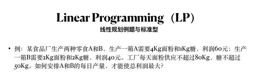
Think before calculating. What are we allowed to choose? What does the workshop want to maximize? Which sentences describe limits rather than preferences?

The quantities we control are the numbers of boxes. Letanddenote those numbers. Profit is not a constraint; it is the score by which we compare feasible production plans. Flour and sugar, on the other hand, are hard limits.

Translate one sentence at a time

The profit from A isand the profit from B is, so total profit is

Now translate the flour sentence. Every A consumes 4 kg and every B consumes 2 kg. The total cannot exceed 80 kg:

Sugar gives a second restriction:

Finally, negative production is meaningless, so. We have now written the complete model:

Notice the order in which we worked: meaning first, symbols second. If you begin by searching for an algorithm, it is surprisingly easy to optimize the wrong problem very efficiently.

Solve it without software

Because there are only two variables, draw the feasible region. The flour boundary isand the sugar boundary is. Their intersection satisfies

Multiply the first equation by two and subtract the second. We obtain, soand then. The profit is

For a linear program, an optimum occurs at a corner of the feasible polygon whenever an optimum exists. The other corners are,, and, with profits 0, 1200, and 1000. Thereforeis indeed optimal.

Read the answer like a modeler

The number 1400 is not the whole conclusion. At, flour usage iskg and sugar usage iskg. Both resources are fully used, which tells us both constraints are binding. If the owner can buy more flour but not more sugar, the value of that purchase depends on how the optimal corner moves. This is the beginning of sensitivity analysis and duality.

There is also a modeling decision hiding in plain sight: can we produce fractional boxes? If the answer is no, thenandmust be integers. We were lucky that the continuous optimum is already integral. In another problem, rounding a fractional optimum can violate a constraint or miss a much better integer plan.

A quick variation

Suppose A earns 80 rather than 60. Do not rerun software immediately. Compare the objective at the corners:now earns 1600, whileearns 1600 as well. The objective line is parallel to the flour boundary, so every feasible point on the segment between those corners is optimal. Multiple optima are not a solver bug; they reveal that the data do not distinguish among several plans.

The opening allocation question tells us what must be chosen and what “better” means. If both the objective and the hard rules can be written as linear expressions, we get a linear program; let us build one from the story before naming a solver.

Let’s test the model against the factory floor

Before we leave the workshop, I want you to try an awkward but useful question: what exactly is a “box”? If one box can be prepared with any nonnegative real quantity of ingredients, our continuous model is a reasonable approximation. If it is a sealed retail package, boxes are indivisible. If the factory produces in batches of ten, the decision should perhaps beandwith integer batch counts. A solver cannot infer this from the word “box.” We have to ask the person running the workshop.

Try a seemingly harmless production plan: 12 boxes of A and 18 of B. Flour consumption iskg, already four kilograms too high. Sugar consumption iskg, perfectly fine. The plan would earnyuan, more than our optimal plan, but it is not feasible. This is a wonderful first lesson in optimization: an impressive objective value is worthless if the plan cannot be implemented. Whenever somebody reports a surprisingly good profit, first recompute the resource totals.

Now try 8 boxes of A and 20 of B. Flour usage iskg; sugar usage iskg; profit isyuan. This is feasible, but leaves eight kilograms of flour and two kilograms of sugar. Would adding a box of A help? It would consume four flour and one sugar, so one extra A is feasible and raises profit to 1340. We can add a second A, reaching our optimal plan. That reasoning is not a full general-purpose algorithm, but it helps a beginner feel the difference between “feasible” and “best feasible.”

The chart of feasible plans is a polygon only because we allowed continuous quantities and the inequalities are linear. If the plan must be integral, picture a grid of candidate points inside the polygon. The best continuous point may land between grid points; we then need to compare nearby legal points, not simply round each coordinate independently. Rounding up both coordinates may step outside the pantry limits, while rounding down can waste resources. In our particular numerical example, the intersection happens to sit on a legal grid point. This coincidence makes the hand calculation especially neat; it should not become a habit of ignoring integrality.

What if the owner asks for a minimum of five boxes of each snack because regular customers expect both? Addand. Do not secretly change the profits. What if the oven can heat only 25 boxes, regardless of recipe? Add. This new rule changes the answer:makes 30 boxes, so it is no longer feasible. A good formulation is allowed to change when the story changes. The point is that each new restriction must have a sentence in the real world that explains it.

Here is another trap: “A earns 60 yuan” may mean revenue, not profit. If raw materials cost money, transport is billed per box, or unsold snacks are returned, maximizing stated revenue is not the same as maximizing net profit. Ask whether 60 and 40 are already net contribution margins. If they are not, subtract variable costs from the objective. An optimization model can be solved exactly while answering the wrong business question, so the meaning of the coefficients deserves as much attention as the equations.

Finally, test the units. The termhas units of kilograms of flour, not yuan; therefore it belongs in a flour constraint. The termhas units of yuan and belongs in the objective. We cannot adddirectly toany more than we can add fifteen minutes to three meters. Dimensional checks sound elementary, yet they catch a surprising number of competition mistakes. When the model grows to dozens of variables, writing units next to every parameter is one of the cheapest forms of quality control.

From linear programs to conic constraints

A linear program has the standard form

The coefficients must be constants. Products such as, ratios of decisions, and squared decisions are not linear.

Why a line stays a line

Let us unpack the word “linear” rather than treating it as a badge. If the production of A increases by one box while B stays fixed, profit rises by 60 yuan, regardless of whether we started at zero A or ten A. Similarly, each extra A always consumes four more kilograms of flour. The marginal effects are constant. That is exactly the assumption encoded by a linear coefficient.

Real factories sometimes violate it. A bulk discount might reduce ingredient cost after the twentieth box; overtime may increase labor cost after a shift threshold; a setup operation may cost money whenever a recipe is produced at all. We can often represent thresholds with additional variables and constraints, but we should not pretend the original two-variable LP already contains them. Start simple, state the assumption, and add complexity only when it changes the decision. A beginner can practice this by asking, “If I produce one more box, does the effect really stay the same everywhere?” If not, the coefficient may need a different model.

The feasible region of an LP is an intersection of half-spaces. In two dimensions we can draw it. In higher dimensions we cannot draw every coordinate at once, but the geometry still tells us something: the feasible set is convex. If two plans each respect every linear resource limit, then every proportional mixture of those plans also respects the same limits, provided fractional mixtures are physically meaningful. To see why, take two flour-feasible plansand, withand. For any, the mixtureusestimes the first flour usage plustimes the second, and this cannot exceed. The same argument works for sugar. We will reuse that simple idea when we reach convexity.

Why did we only check corners for the snack LP? Imagine sliding a straight line representing constant profit across the feasible polygon. We slide it toward higher profit until it touches the polygon for the last time. That last touch occurs at a vertex, unless the line lies along an edge, in which case every point on the touched edge shares the same optimum. Our variation with A earning 80 yuan produced exactly such an edge of equally good answers. The geometry also explains why changing profits can suddenly switch the preferred production mix: the objective line changes its slope and may touch a different corner.

This picture is powerful but has boundaries. A linear objective on an empty feasible set has no answer. If a direction lets profit grow without limit because a resource constraint is missing, the model is unbounded. If the model contains integer variables, the continuous polygon is only a relaxation. The first three solver statuses you should understand are therefore optimal, infeasible, and unbounded. Do not read “infeasible” as “the algorithm failed”; it may be telling you that the rules conflict. Do not read “unbounded” as “unlimited real profit”; it may reveal a missing limit in your formulation.

Take a tiny infeasible variant: the owner demands at least 30 boxes of A while flour remains at 80 kg. Thirty A alone require 120 kg flour. No arrangement of B can repair that. The solver should report infeasibility, and we can explain it in one sentence to the owner. Take a tiny unbounded variant: remove both resource limits but keep positive profit coefficients and nonnegative production. The mathematical answer is to make arbitrarily many boxes. Real production cannot do this, so the model must be missing capacity, time, or demand limits. This is why status messages can be diagnostic evidence about the story rather than merely about the software.

A resource is valuable only in context

At, both ingredient constraints bind. Suppose the owner can acquire one extra kilogram of flour at a cost of ten yuan. Would we buy it? We need the marginal value of flour in the current production regime. Letandbe the yuan values of one extra kilogram of flour and sugar. At the optimal mix, the value of ingredients used by each produced snack equals that snack’s contribution margin:

The second equation says; substitute into the first to get. Thusyuan/kg andyuan/kg. If the extra flour really costs ten yuan/kg and we may change the production mix fractionally, a small purchase can increase gross optimal profit by roughly 13.33 yuan and net profit by about 3.33 yuan. If flour costs fifteen yuan/kg, a small purchase is not justified by this local calculation. If we can only buy flour in truckloads or produce whole boxes, we must resolve the discrete model instead of extrapolating this derivative.

There is an important qualification: the numbers 13.33 and 6.67 are local. As we add flour, the optimal mix changes; eventually one resource or one product may cease to be active, and the marginal value changes. A shadow price is a slope of the optimal-value curve near the current data, not a promise that a thousand extra kilograms will be equally valuable. This is why sensitivity intervals or fresh solves matter. You can explain the same point in ordinary language: the first extra flour kilogram may be useful because sugar still exists to turn it into snacks; after enough flour arrives, sugar becomes the only bottleneck.

What if the owner can buy additional sugar for five yuan/kg? Its local value is about 6.67 yuan/kg, so a very small purchase also looks worthwhile. But if the owner can buy either flour or sugar under a fixed cash budget, compare net value per yuan spent, consider integer batches, and test how far the local approximation remains valid. The dual values guide a conversation; they do not replace the new decision model. This is the bridge from finding an optimum to using an optimum.

For two products with profitsand, flour useand, sugar useand, and capacitiesand,

subject to

If boxes must be whole, the variables are integer and the problem becomes a mixed-integer linear program. Do not solve the continuous relaxation and round blindly: rounding can violate constraints or destroy optimality.

Assignment and logical decisions

Letwhen taskis assigned to worker. A minimum-cost assignment is

with

Binary variables also encode activation, ordering, coverage, and incompatibility. If alternativesandcannot coexist, use. If selecting projectrequires facility, use.

Quadratic programs

A quadratic program uses

with linear constraints. It is convex when. Quadratic terms naturally represent squared tracking error, variance, smoothness, and distance-like penalties.

Portfolio selection is a canonical example:

Herecontains portfolio weights,is the covariance matrix, andis expected return. The covariance estimate—not the optimizer—often dominates the model’s uncertainty.

Conic structure

Second-order cone constraints have the form

They represent norm bounds, robust linear constraints, and many risk limits. Recognizing convex structure matters because a convex feasible problem has no misleading local optimum: solver certificates and dual information become meaningful.

Formulation workflow

Write the model in this order:

1. indices and sets;
2. known parameters and units;
3. decision variables and domains;
4. objective, with each term interpreted;
5. constraints, grouped by real rule;
6. solver and numerical tolerances;
7. post-solve feasibility and sensitivity checks.

Scale coefficients when one part of the model is nearand another near. Poor scaling can make a correct formulation numerically fragile.

Interpreting the solution

Report active constraints, unused capacity, and marginal values—not only. A dual variable estimates how the optimal objective changes when the corresponding constraint is relaxed slightly. It can identify the resource worth purchasing next.

SciPy’s official linprog interface uses exactly the inequality, equality, and bound form above and currently delegates to HiGHS methods (documentation ). After solving, independently recompute the objective, integrality, and every constraint from the returned decisions.

For the snack example, SciPy minimizes, so negate the profit coefficients:

import numpy as np
from scipy.optimize import linprog

c = np.array([-60.0, -40.0])
A = np.array([[4.0, 2.0], [1.0, 2.0]])
b = np.array([80.0, 50.0])

result = linprog(c, A_ub=A, b_ub=b, bounds=[(0, None), (0, None)])
assert result.success
x = result.x
profit = -result.fun
violation = np.maximum(A @ x - b, 0).max()
print(x, profit, violation)

Read the answer in domain language: how many boxes of each product, expected profit, which resource is binding, and whether continuous quantities are physically allowed. If boxes must be integral, use a mixed-integer solver instead of this continuous model.

Worked problem: assigning students to projects

Linear programming becomes much more expressive when the decisions are yes-or-no choices. Here is a complete assignment problem, not merely the final formula.

The slide states the general assignment problem. Our three-student table below turns the indices into a small instance that we can solve completely by hand.

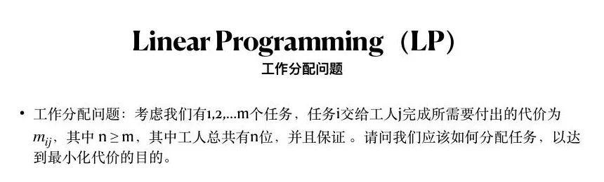
The question

Three students—Ada, Ben, and Chen—must each receive one of three projects: Vision, Planning, and Control. Their estimated completion times in hours are

Student	Vision	Planning	Control
Ada	6	9	7
Ben	8	5	6
Chen	7	8	4

Every project must be assigned exactly once. Find the assignment with the smallest total time.

Before the solution: there are only six possible assignments, so we could enumerate them. Why build a model? Because the model will still work when there are 300 students, eligibility rules, workloads, and team constraints.

Choose a representation

Letif studentreceives project, and let it be zero otherwise. The phrase “Ada receives Vision” is no longer a vague sentence; it is the event.

The total time is the sum of time multiplied by the corresponding selection indicator:

Each student gets exactly one project,

and each project is used exactly once,

Finally,. Do not omit the binary domain. If we merely require, the symbols could mean fractional assignments. The classical square assignment problem happens to have an integral LP relaxation, but that is a mathematical property of this constraint matrix—not permission to forget what the variables mean.

Solve and explain

Choosing Ada–Vision, Ben–Planning, and Chen–Control giveshours. Checking the remaining five permutations gives totals 20, 21, 22, 23, and 19 hours, so 15 is optimal.

The useful answer is not “the solver returned 15.” It is: Ada should take Vision, Ben Planning, and Chen Control; every student and every project appears once; and the predicted workload is 15 hours. If the time estimates are uncertain, perturb them and see whether the same assignment remains optimal. A plan that changes after a one-hour estimation error is much less trustworthy than one that survives all plausible estimates.

Add real rules

Suppose Ada is not certified for Control. Set. Suppose Ben and Chen cannot work on Planning and Control simultaneously because those projects share equipment. One possible rule is

Read that inequality aloud: at most one of the two named events can occur. This habit catches logical mistakes faster than staring at indices.

Now suppose a student can take two small projects but at most 12 hours of predicted work. Replace “one project per student” with

The same binary language supports scheduling, facility opening, feature selection, set cover, and routing. The algorithm may change, but the modeling habit stays the same.

Why the assignment is not three separate choices

Let’s slow down at the point that usually trips up a first-time reader. Ada’s fastest project is Vision at six hours. Ben’s fastest is Planning at five hours. Chen’s fastest is Control at four hours. In our invented table those individual favorites happen to fit together, so the greedy choice gives the optimum. But that happy outcome is not a theorem. If Ada and Ben both favor Vision, only one of them may receive it. The cost of giving Vision to Ada includes an opportunity cost: what does Ben do instead? This coupling is why the constraint “each project exactly once” is not decorative.

To make that visible, change only Ben’s Vision estimate from eight hours to three hours. His preferred project is now Vision, and Ada still prefers Vision at six. If we give Vision to Ada, Planning to Ben, and Control to Chen, the total remains fifteen hours. If we give Vision to Ben, the best legal way to place Ada and Chen may be Ada–Planning at nine and Chen–Control at four, totaling sixteen hours, or Ada–Control at seven and Chen–Planning at eight, totaling eighteen hours. The individually fastest-looking Ben–Vision option is not the globally fastest complete assignment. We should compare whole plans, not rank each row in isolation.

Here is a small exercise worth doing with pencil. List the six permutations explicitly:,,,,, and, where the three positions refer to Ada, Ben, Chen. For the original table, their totals are respectively. The fifth line is not “close enough” merely because every individual cost looks reasonable. Enumeration is a good benchmark for a three-person problem; with thirty people it becomes impractical, which is why the mathematical structure matters.

What if one task takes two people rather than one? The right model depends on what “takes two” means. If two workers independently contribute to the same task, change that task’s coverage equation to. If the two workers must be a compatible team and the cost depends on the pair, worker-task binary indicators may not be enough; add pair variables and coupling constraints. If a worker can take two tasks provided total hours stay below twelve, use a workload constraint. We never get these rules by staring at a cost table. We get them by interviewing the real assignment process.

Now return to the certification and shared-equipment constraints. Ada not certified for Control deletes two of the six permutations. The incompatibility ruledeletes our former optimum because both indicators are one. Among the remaining legal assignments, Ada–Vision, Ben–Control, Chen–Planning costshours, while Ada–Planning, Ben–Vision, Chen–Control costs; the other legal candidates cost more. So the extra rule raises the best predicted time from 15 to 20 hours. That five-hour increase is not “inefficiency introduced by the solver.” It is the cost of enforcing a business rule we did not include before.

This example suggests a way to test any binary constraint. Construct a plan that should be legal and a plan that should be illegal. Substitute their zero-one values into the inequality. If the first is rejected or the second is accepted, the encoding is wrong. For “if A then B,” write all four possibilities: no A/no B, no A/yes B, yes A/no B, yes A/yes B. The inequalityrejects only yes A/no B. A truth table is not childish; it is a compact proof that the model says what we intend.

What if completion times are only guesses?

Suppose Ada’s Vision estimate might be anywhere from six to ten hours depending on how much image-labeling work arrives. Our 15-hour plan could then take as long as 19 hours. The alternative Ada–Control, Ben–Planning, Chen–Vision currently takes 19 hours. Under some plausible cost changes it may become preferable. We should not report “Ada must take Vision” as a universal truth. We should report the assumptions and ask how stable the assignment is across scenarios.

A simple sensitivity experiment changes one table entry at a time. Increase Ada–Vision from six to seven, eight, nine, and ten, re-solve, and mark the first value at which the preferred assignment changes. Then test simultaneous changes, because real delays are often correlated: a complicated project may delay several students. You can show a small heat map of assignments across scenarios rather than a single hard-to-read table of solver statuses. The lesson is not that uncertainty forces a complicated algorithm. It is that a result computed from estimates should be spoken about as an estimate.

There is one more subtle point about the assignment LP. If every student receives exactly one project and every project exactly one student, the linear relaxation withhas an integral extreme-point optimum. This comes from the structure of the matching constraints. It does not mean every model with binary variables becomes integral after dropping integrality. Add a shared-equipment rule, team rule, or fixed-opening cost, and the useful guarantee may disappear. Explain the distinction this way to a beginner: some constraint systems are specially shaped so that a continuous solver naturally lands on whole choices; others are not. We can exploit that special structure when it applies, but we still define the decisions correctly and verify the returned values.

The snack decision used continuous quantities, and this assignment uses discrete yes-or-no choices. Both are ways to coordinate limited resources. The next case adds geography: there are several recipients, two suppliers, and route distances. First the supplier positions are fixed, so the optimization remains linear. Then we let the suppliers move and watch why the mathematical structure changes.

Worked problem: locating supply depots

This example from the course is especially useful because it shows how a small change in the question can change the entire mathematical class of the problem.

The full supply-and-location prompt, including the six coordinates and daily demands. We solve the fixed-depot allocation first, then explain why movable depots change the model class.

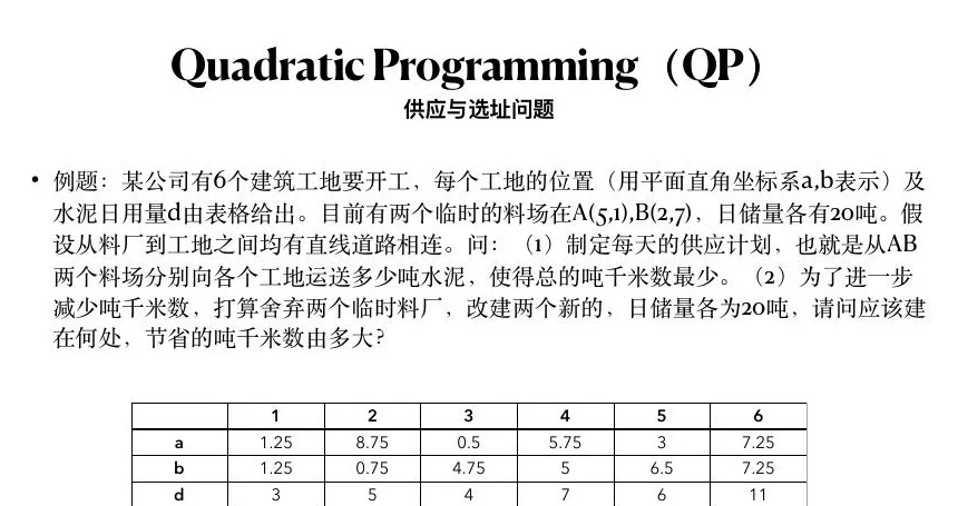
The fixed-depot question

There are six construction sites with coordinates and demands:

Site	1	2	3	4	5	6
	1.25	8.75	0.50	5.75	3.00	7.25
	1.25	0.75	4.75	5.00	6.50	7.25
Demand	3	5	4	7	6	11

Two existing depots are atand, each with 20 tons of stock. We must determine how much material each depot sends to each site while minimizing ton-kilometers.

Take a moment to identify what is fixed. The site coordinates, depot coordinates, site demands, and depot capacities are data. The shipment quantities are decisions. Therefore letdenote tons shipped from depotto site. The distance coefficient

is a constant becauseis fixed. The model is

subject to demand balance

and depot capacity

This is a transportation LP. Total demand istons and total supply is 40 tons, so aggregate capacity is sufficient. That does not yet prove feasibility when there are forbidden routes, but with every route available it gives a useful first check.

Read the map before solving

Let’s walk around the map as if we were arranging deliveries on a whiteboard. Six sites need a total of 36 tons each day. Two depots together can provide 40 tons. That leaves four tons of aggregate spare capacity, but the spare capacity is not one big anonymous pool: each individual depot has only 20 tons. If we accidentally write just, we could ask depot B to supply 30 tons and pretend that depot A’s unused stock magically appears at B. The two capacity inequalities are not optional bookkeeping; they preserve the physical location of the inventory.

The coordinates are measured in some unit of distance. If they are kilometers, a shipment of three tons over a five-kilometer route contributes fifteen ton-kilometers. If the coordinates are map-grid units rather than kilometers, do not call the objective literal ton-kilometers until you know the scale. The model is still valid as a comparative distance-weighted cost if all routes use the same grid. This is one of those small questions that makes the final explanation honest.

Before opening any software, compute a few distances to see whether the numbers make sense. For site 1 at, the distance from A atis approximately; the distance from B atis approximately. A is closer. For site 5 at, the distance from A is approximatelyand from B approximately. B is much closer. Site 4 atis nearly equidistant: aboutfrom A andfrom B. A small data or route-cost correction could reverse its apparent preference. That observation tells us where sensitivity might matter after the nominal optimum.

The exact Euclidean formula assumes trucks travel in straight lines. Real road travel may be longer, may depend on traffic, and may have one-way restrictions. If we have a road network and travel-time data, replace each straight-line coefficientwith the appropriate measured or shortest-path cost. The flow model stays linear as long as those route coefficients are fixed. The numerical answer may change. This distinction is useful: bad distance data are not repaired by a more powerful optimizer, while better route data do not necessarily require a more complicated decision model.

Why the nearest-depot rule can fail

A tempting shortcut is to send every site’s demand to the nearest depot. Try it. If too many sites choose the same depot, its 20-ton capacity may be exceeded. A locally cheapest choice for each site need not be globally feasible. The LP coordinates all shipments at once and can split a site’s demand if that lowers cost or restores feasibility.

Let’s do the shortcut completely rather than merely warning against it. With the stated coordinates, A is closer to sites 1, 2, and 4, whose demands aretons. B is closer to sites 3, 5, and 6, whose demands aretons. So the nearest-depot plan asks B to ship one ton beyond its available stock. The total 36-ton demand is below the combined 40-ton supply, but the particular route selection is infeasible. This is a tiny example of a global constraint defeating a series of local choices.

Which ton should move from B’s nearest-depot group to A? Compute the additional distance per ton for each candidate. For site 3, A is aboutunits farther. For site 5, A is aboutfarther. For site 6, A is aboutfarther. Moving one ton of site 6’s delivery from B to A has the smallest incremental cost among those three direct repairs. The resulting shipments are: A supplies all of sites 1, 2, and 4 plus one ton to site 6, totaling 16 tons; B supplies all of sites 3 and 5 plus ten tons to site 6, totaling 20 tons. Every site receives its complete demand and both depots stay within stock.

The all-nearest plan’s distance-weighted sum is aboutton-distance units, but it cannot be executed. Our repaired plan costs aboutunits. A transportation solver can confirm the optimum by comparing all legal flow exchanges; for this small fully connected instance, this one-ton repair is indeed the cheapest way to relieve B’s capacity, because each displaced B ton incurs at leastadditional distance. Notice the wording: we compare a feasible optimum with a hypothetical infeasible lower-cost plan. We should not presentas a genuine alternative policy for the company.

What if split deliveries are prohibited? Then the repaired plan, which divides site 6’s shipment between depots, is illegal. We need a binary assignment variable saying which depot serves a site, link flow to that assignment, and re-solve a mixed-integer model. Site 6 has eleven tons of demand, so moving all of its deliveries to A would load A with 26 tons and violate capacity. Moving site 3’s four tons to A would give A 19 and B 17, but it adds aboutdistance units relative to the all-nearest map. There may be another whole-site shift that is cheaper; enumerate all feasible site assignments or use a MILP to check. The central lesson is that one sentence, “a site may receive trucks from both depots,” determines whether a continuous split-flow plan is acceptable.

The LP also assumes all demand must be met exactly. If deliveries may be delayed, introduce unmet-demand variables with a justified penalty. If surplus deliveries can be stored at a site, change the equality to an inventory balance over time rather than silently allowing overdelivery. If capacity resets daily, the model applies separately each day; if unused stock carries over, the state of the depot must be linked across dates. These are not details for a solver manual. They are the questions that make the result operational.

After solving, draw only the routes with positive flow and label their tonnage. Then independently check three things: each site receives exactly its demand, neither depot ships more than 20 tons, and the displayed objective equals the sum of distance times flow. This small audit is more persuasive than a screenshot of solver output.

Now allow the depots to move

Suppose the question changes: where should the two depots be located? The coordinatesbecome decision variables. The distanceis no longer a constant; it now depends on those decisions:

The productcouples location and allocation. The clean transportation LP has become a nonlinear location-allocation problem. This is a perfect example of why we classify the model after defining the variables. The same-looking map may represent an LP, a mixed-integer facility-location model, or a nonconvex continuous location problem.

One practical baseline alternates two steps:

1. hold depot locations fixed and solve the transportation LP;
2. hold allocations fixed and update each depot location using its assigned weighted points.

The objective cannot increase if each step is solved correctly, but the procedure can settle at a local solution. Use several starting locations, compare with a simple grid search for a small instance, and report how sensitive the final configuration is to initialization.

Understand what changed mathematically

For a fixed depot at, the cost of sending one ton to site 1 is a known number, aboutdistance units. We may writein a linear objective. If the depot itself can move, its locationis unknown. The same term becomes. Both the flow and the distance are decisions, and their product is not generally convex in the joint variables. Do not reason “distance is a norm, norms are convex, therefore the entire model is convex.” A nonnegative fixed weight times a norm is convex in location; a decision-dependent weight times a decision-dependent norm need not be.

We can make this distinction tangible with two simpler questions. If every site is permanently assigned to A and the delivered quantities are fixed, choosing A’s coordinates to minimize the weighted sum of distances is a geometric-median-type problem; the objective is convex in A’s coordinates. If A and B have fixed coordinates, choosing shipment flows is the transportation LP we just solved. When both assignments/flows and coordinates vary together, the separate nice structures do not automatically combine into one convex problem. This is why alternation is reasonable as a heuristic: it temporarily restores one easy subproblem at a time. It is also why one alternating run is not a global-optimality certificate.

Suppose there are two plausible initial location pairs: near the two old depots, and near clusters of high-demand sites. Solve the alternating method from both. If the final objectives differ, we have direct evidence of initialization sensitivity. If they match, that is encouraging but not a proof of a unique global optimum; perhaps both starts fell into the same basin. For six sites we might perform a coarse grid search, solve the allocation LP at each grid point, then refine promising locations. For a larger instance we might use multistart, specialized location algorithms, or a mixed-integer discrete-candidate formulation. The choice depends on the required guarantee, the size of the candidate region, and the time available.

The 20-ton stocks can also change when depots move. Are we relocating warehouses and their existing inventory, building new facilities, or deciding tomorrow’s loading points? If a new depot must be built, add construction cost and perhaps zoning restrictions. If stock at old depots remains physically there, a solution that simply moves the coordinate labels would be nonsense. The course exercise asks us to minimize transport work, but a practical recommendation should distinguish transport savings from total project economics. A model can be perfectly solved and still omit the cost that decides whether relocation is worthwhile.

We now have three related optimization languages: quantity choice at a factory, yes-or-no assignment of people, and distance-weighted flows on a map. Their common thread is that the objective must be evaluated only for plans respecting all constraints. In the next case, the objective itself becomes curved because spreading an investment across assets changes risk in a way that depends on how the assets move together.

What to report

Coordinates alone are not a decision story. Report the original and optimized ton-kilometers, percentage saving, utilization of each depot, routes that change, and whether a small demand perturbation changes the recommended sites. If building a new depot costs money, add that cost before declaring relocation worthwhile.

Worked problem: balancing return and risk

Quadratic programming is easiest to understand through a trade-off that linear terms cannot express naturally.

The question

An investor allocates proportionsamong three assets. The weights sum to one and short selling is not allowed. Expected returns are stored in, and the covariance matrixdescribes how returns vary together. We want the least risky portfolio that still reaches target return.

First, let’s say plainly what is being chosen. A weight ofmeans forty percent of the available capital goes to asset 1. If we invest all available capital, the weights add to one. If borrowing or short selling are forbidden, each weight is nonnegative. Expected return is an estimate of the average gain over a declared time horizon; it is not money guaranteed to appear. A covariance describes whether two assets tend to surprise us in the same direction or in opposite directions. This is why a risk model needs more than a column of individual standard deviations.

Risk is modeled by portfolio variance. Thus

Build variance from a two-asset toy example

Before acceptingas a mysterious matrix formula, consider two assets with annual-return standard deviations ofand. Their variances areand. Suppose their correlation is. Their covariance is. If we place half the money in each, portfolio variance is

The corresponding standard deviation is. That is lower than either individual standard deviation because the assets tend to move against each other. If we had used only an average of the individual variances, we would have missed the negative cross term. If the correlation were positive instead, the cross term would raise risk. The covariance matrix is just a compact way to gather all of these pairwise effects for three, ten, or a hundred assets.

Does an 8.66% standard deviation mean the portfolio will lose no more than 8.66% in a year? No. Standard deviation summarizes a distribution; it is not a hard loss ceiling, and the quality of the estimate depends on the data and assumptions. A course solution should keep that statistical interpretation separate from the optimization guarantee. Convexity can tell us that we found the minimum of the specified estimated-variance objective under the specified constraints. It cannot tell us that the future behaves like the past.

Now think about the target-return rule. If we require a return larger than every asset’s estimated return and do not allow leverage, the constraint is impossible. The optimizer’s infeasible status is then understandable: a weighted average of numbers cannot exceed their maximum. If we require a very modest return, the target may be inactive, and the optimizer may choose the lowest-variance combination regardless of return. If we raise the target, the feasible portfolios shrink and the minimum achievable variance usually rises. Solve at several target levels and draw the resulting return–risk frontier. Each point answers a distinct decision question; none is universally “best” until the decision maker states how much return matters.

The no-short-selling rule also affects geometry. Without, a solver could assign a negative weight to an asset, meaning a short position financed by other positions. Short selling might be allowed in some markets, but it brings borrowing costs, collateral, and risk. We cannot silently allow it just because a mathematical minimum looks appealing. The same principle applied to indivisible snack boxes: the domain of a variable is a statement about permitted actions.

Think first: why not minimize the average of the three individual variances? Because covariance matters. Two volatile assets can partially cancel one another if they move differently, while two apparently safe assets can reinforce the same risk.

Convexity is a promise

A covariance matrix is positive semidefinite in exact mathematics, so the variance objective is convex. Geometrically, its level sets are ellipses rather than a landscape full of unrelated valleys. If the constraints are also convex, every local optimum is global. This does not mean every numerical answer is automatically meaningful: estimated covariance can be noisy, the target return can be infeasible, and tiny eigenvalues can make the solution unstable.

Check thatis symmetric and inspect its eigenvalues. If sampling noise produces a small negative eigenvalue, investigate the preprocessing or use a justified positive-semidefinite correction. Then solve several target returns to trace an efficient frontier. The frontier communicates the trade-off far better than one unexplained portfolio.

The reason a covariance matrix should be positive semidefinite is almost elementary. For any portfolio weight vector, the quantityrepresents the variance of a weighted combination of returns. A variance cannot be negative. Thereforefor every. A sample-covariance matrix calculated consistently from the same observations has this property, although estimation and numerical approximations can leave tiny negative eigenvalues. If you see a large negative eigenvalue, do not quietly clip it and move on. Check whether you mixed incompatible time windows, used correlations as covariances, or changed units between assets.

Portfolio variance is a quadratic objective. Its gradient changes with, unlike the constant profit gradient in the snack LP. As the portfolio weights move, the incremental risk of adding one asset depends on the other weights. This is the source of the curve in the efficient frontier. The model remains convex whenis positive semidefinite and the return, budget, and nonnegativity constraints are linear. In other words, a curved objective is not automatically a dangerous objective. The relevant question is whether it curves in the right direction for minimization.

Interpret the result

Suppose the target-return constraint is active. Its dual value measures the local increase in minimum variance caused by demanding slightly more expected return. If the dual value is large, the investor is near a costly part of the frontier. If a weight is zero, its reduced-cost or KKT condition explains why that asset does not enter the current optimum.

Finally, validate out of sample. A portfolio optimized on the same period used to estimateandwill usually appear too good. Roll the estimation window forward, include transaction costs, and compare with equal weights. Optimization should earn its complexity against that baseline.

Imagine reporting three weights to a classmate and saying, “The model selected these because they minimize estimated variance while meeting a ten-percent target return.” Your classmate asks, “What if the estimated return of asset 2 was overoptimistic?” That is the right challenge. Re-estimate returns from a different period, perturb the most uncertain mean, or optimize under several plausible scenarios. If the chosen weights jump from nearly zero to nearly one under a tiny perturbation, report the instability. A mathematically global optimum can be practically fragile. That distinction between optimization accuracy and input uncertainty will lead naturally to our next lesson about multi-objective and robust decisions.

Where a cone enters the story

The course also introduces second-order cone programs. A beginner can understand the core constraint without learning conic geometry all at once. Suppose a robot’s estimated position error is a two-component vector. We want its Euclidean magnitude to stay below a tolerance:. Writing this assays exactly the same thing. If the error vector is an affine expressionin the decisions and the tolerance is an affine expressionthat stays nonnegative, we have a second-order cone constraint.

Picture a circle of allowed error vectors in two dimensions. The circular boundary is curved, but the feasible set inside it is convex: average any two allowed error vectors and their average is still allowed. This is very different from requiring the error to be at least, which would put us outside a circle and make mixtures of two opposite feasible points potentially infeasible. The direction of the inequality determines whether the curved rule is safe for convex optimization.

One common robust-optimization interpretation is this: a constraint must hold for every coefficient perturbation inside a Euclidean uncertainty ball. Instead of enumerating infinitely many perturbations, the worst-case linear effect may be written as a norm of a decision-dependent vector. That reformulation can give a cone inequality. But do not label every vague claim about uncertainty “SOCP.” State the uncertainty set, derive or justify the worst-case bound, and check whether the resulting right-hand side is nonnegative. Our purpose is not to collect solver acronyms; it is to give the physical uncertainty a valid mathematical shape.

Assignment, depot location, and return–risk balance look like different problems. The unifying question is whether a local best point can also be a global best under the declared feasible set. That is why we now examine convexity, not as vocabulary but as a guarantee about the search.

Convexity clinic: how to recognize the safe structure

Course formulation exercises. Before looking for a solver, identify the variables and decide whether each objective and feasible set is linear, quadratic, conic, or nonconvex.

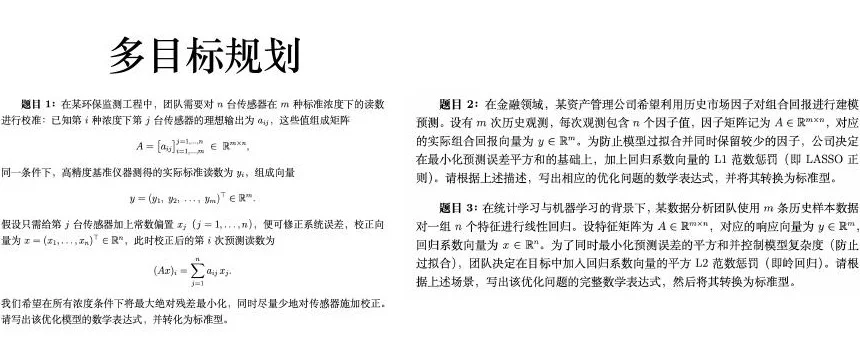
When we call a problem convex, we are making two statements:

• the feasible set contains the whole line segment between any two feasible points;
• the objective lies below the chord connecting any two points on its graph.

For a differentiable function, the first-order condition

means that every tangent plane is a global under-estimator. For twice-differentiable, a positive-semidefinite Hessian is a convenient test. Linear functions are both convex and concave; norms are convex; the maximum of convex functions is convex; an arbitrary product of variables usually is not.

Here is a useful classroom test. Consider each expression and decide before reading the answer:

1. — a half-space, hence convex.
2. — a disk, hence convex.
3. — the outside of a disk, not convex.
4. with— despite the product, this particular feasible set is convex: it is the epigraph, andis convex on. Do not classify a set from syntax alone.
5. — a second-order cone constraint when the right side is nonnegative.

The direction of an inequality matters. A convex function bounded above defines a convex sublevel set; the same function bounded below generally does not.

Test the guarantee rather than memorizing the label

We should be precise about the two ingredients of a convex minimization problem. A convex objective is not enough if the permitted decisions form a disconnected set. A convex feasible region is not enough if the objective has two separated valleys. Both properties work together to make a local optimum global. In our snack LP, linear inequalities make a convex polygon and linear profit is both convex and concave; maximizing linear profit over that polygon is equivalent to minimizing its negative, also linear. In the assignment problem, the zero-one decisions break the continuous line-segment property: the average of two legal binary assignments is generally fractional and not a legal assignment. In the portfolio QP, both the variance objective and the simple allocation rules have the right convex shape, provided the covariance estimate is positive semidefinite.

Take the simplest objective. Atand, the value is four. At their midpoint,, the value is zero, below the straight chord joining the two endpoint values. That is the visual meaning of convexity. More generally, for, convexity asks for. The right side is the value on the chord; the left side is the value on the graph at the mixed point. The function is allowed to be curved. It simply may not rise above the chord.

Now look back at the feasible-set testwith both coordinates positive. A quick “products are nonlinear, therefore nonconvex” verdict would be wrong. Rewrite it asfor. Becauseis convex there, the region above its curve is convex. We do not need to claim the constraint is an LP; it is not. We only need to distinguish linearity, convexity, and representability by a particular solver form. These are related but not identical ideas. This distinction matters in a lesson titled convex optimization: students should be able to diagnose the actual shape, not just repeat a list of forbidden symbols.

When a rule contains a norm, test the whole rule.is a standard convex cone constraint on its proper domain. If we reverse it to, the region can be nonconvex. If we make the right side a nonlinear uncertain expression, more analysis is needed. If we add an “open this facility or not” binary choice, the full problem is mixed-integer even if every continuous subproblem is convex. Each change in the story can change the guarantee. That is why we classify after writing variables and constraints.

From optimality conditions to explanation

For a constrained convex problem, the Karush–Kuhn–Tucker conditions connect the numerical optimum to a human explanation. Introduce one multiplier for each constraint. At the optimum we look for:

1. primal feasibility — the decisions satisfy the original rules;
2. dual feasibility — inequality multipliers have the correct sign;
3. stationarity — objective and active-constraint gradients balance;
4. complementary slackness — an inactive inequality has zero multiplier.

In the snack problem, both ingredient constraints are active. Their multipliers can be interpreted as marginal values of flour and sugar. If sugar had 10 kg left unused, complementary slackness would force its shadow price to zero locally: one more kilogram of an already abundant resource cannot improve profit. For the stated data, the dual values are approximately 13.33 yuan per extra kilogram of flour and 6.67 yuan per extra kilogram of sugar, within the range over which the same production basis remains optimal. Flour, not sugar, has the higher local marginal value here.

This language helps us explain a solver result without pretending the solver is an oracle. “The plan uses all available flour and sugar; the marginal values show sugar is currently more valuable; product B remains in the mix because it converts flour into profit more efficiently” is a modeling conclusion. “Status: optimal” is only a software message.

From linear programs to networks

Optimization becomes easier when every symbol answers a physical question. Consider shipping a product from factoriesthrough warehousesto customers. Letandbe shipped quantities andtheir unit costs.

Write balance equations

At warehouse, incoming and outgoing flow must balance unless inventory is explicitly modeled:

Factory capacity gives; customer demand gives. The objective is

This is a minimum-cost flow structure. Recognizing structure matters because specialized algorithms are fast and the resulting solution has an interpretable network.

A small warehouse story with actual quantities

Imagine a factory that can ship at most twelve crates tomorrow. There are two warehouses, East and West, each able to handle eight crates. Two customers need five and seven crates respectively. The total customer demand is twelve, exactly equal to the factory’s capacity, so every crate produced must reach a customer. Suppose the factory-to-East shipping cost is 2 yuan per crate and factory-to-West cost is 1 yuan per crate. From East to customer 1 the cost is 1, and to customer 2 it is 5. From West to customer 1 the cost is 4, and to customer 2 it is 1. We can see the route tendencies before writing code: customer 1 is cheaper through East, and customer 2 through West.

Letandbe the numbers of crates entering each warehouse. Letbe outgoing quantities. Warehouse conservation saysand. Customer requirements sayand. Warehouse limits say, and factory capacity says. All quantities are nonnegative. These equations are not a magic flow template: they say that crates cannot appear or vanish between the loading dock and customers.

What does a natural plan look like? Send five crates through East to customer 1 and seven through West to customer 2. East receives five, West receives seven, so both stay below eight. The factory sends twelve. The total cost isyuan. Try moving one crate for customer 1 from East to West. Its route cost rises fromto, so total cost rises by two yuan. Try moving one crate for customer 2 from West to East. Its route cost rises fromto, so total cost rises by five yuan. Because the unconstrained cheapest route plan already satisfies capacities, these more expensive switches cannot help. We have a complete hand-checkable optimum for this tiny case.

Now change West’s handling capacity from eight to six. The original seven-crate delivery through West violates capacity. At least one customer-2 crate must go through East. The repaired plan sends five customer-1 crates and one customer-2 crate via East, and six customer-2 crates via West. East handles six, West six; customer demand and factory capacity still balance. Its cost isyuan. The five-yuan increase is the cost of the first capacity loss under this toy data. If West drops further, each extra customer-2 crate rerouted to East adds five yuan until East’s eight-crate limit binds. Once West can handle fewer than four crates, the two warehouses together can handle fewer than the twelve crates customers require, so changing the customer routes cannot restore feasibility; demand must be relaxed or capacity added. A shadow value has a clear operational story only within such a local range.

This exercise also explains why we separate flow conservation from capacity. The equationprevents disappearance, whileprevents overloading. A student who writes only the capacity rule may let customer delivery exceed incoming stock. A student who writes only conservation may send a legal amount through an impossible warehouse. Both checks are necessary; each answers a different physical question.

There is a useful third check: sum the two customer balances to get twelve required crates, and sum the two warehouse balances to get twelve outgoing crates. The factory balance should then show twelve incoming crates, too. If those totals disagree, inspect an omitted route, a duplicated customer, or a mistaken inequality sign before calling the result optimal. Conservation at each node is stronger than a single total-balance check, but the total is a fast way to locate a problem. In a large network, both local and aggregate audits are worth keeping.

If crates are indivisible, would the continuous LP solution still make sense? In this particular integer-data network flow problem, the classical flow structure has integral optimal extreme points under standard conditions. But if we add a fixed cost for opening East, a minimum shipment size, or a yes-or-no routing rule, the continuous relaxation can propose fractional openings or other impossible behavior. Structure is a tool to exploit, not permission to forget the real decision domain. Test what the factory actually permits and verify that every returned shipment is a whole crate when that is required.

Add discrete decisions carefully

If a warehouse must be either open or closed, introduceand link flow to that decision:

Chooseas the tightest valid capacity, not an enormous arbitrary number. An unnecessarily large big-weakens the relaxation and can create numerical problems. Fixed opening costenters the objective. The model is now mixed-integer and convexity of the continuous part no longer guarantees that a local relaxation solution is an integer optimum.

Logical statements can often be encoded similarly. “Choose at most one of A and B” becomes. “If A then B” becomes. Write a truth table before translating a complicated rule.

Learn the major graph templates

Many competition problems reduce to a few network patterns:

• shortest path: minimum additive cost from a source to a destination;
• maximum flow: greatest feasible flow under edge capacities;
• minimum spanning tree: connect all nodes with minimum total edge weight;
• matching/assignment: pair two sets while respecting exclusivity;
• facility location: choose nodes to open and assign demand to them;
• vehicle routing: construct capacity- and time-constrained tours.

Do not use Dijkstra’s algorithm when edges can have negative costs; do not use a spanning tree when traffic must travel from a source to destinations; do not confuse straight-line distance with travel time on a road network.

Use dual information

Suppose the dual value of factory capacity isdollars per additional unit. Locally, increasing capacity by one unit improves the optimal objective by aboutuntil the active set changes. Reduced costs help explain why unused routes remain unused. Sensitivity ranges are local; after a constraint becomes inactive or another becomes binding, resolve the model.

Diagnose infeasibility

When no solution exists, do not immediately remove constraints. Check units, signs, index ranges, duplicated demand, and lower bounds. Introduce labeled nonnegative slack variables temporarily and penalize them heavily. The locations of unavoidable slack reveal which business rules conflict. Then decide with the domain owner which rule is wrong or negotiable.

Return to the little warehouse instance and imagine the factory can make only ten crates while the customers still require five plus seven. The equality demand rules demand twelve crates. The factory can supply ten. No solver can turn ten into twelve. A useful diagnostic message would tell us that two crates of demand cannot be served under the current rules. We might introduce shortage variableswith customer balancesand. But shortages represent a new business possibility, not a technical patch. The owner must decide whether the model is allowed to miss a customer order, what penalty or priority applies, and whether backorders are possible. If orders are legally mandatory, the model’s infeasible conclusion is itself important: more supply or revised promises are required.

The same diagnosis works for snack production. A minimum production contract can exceed ingredient supply. It works for assignments: three projects may require four certified workers. It works for portfolio targets: an impossible expected return can be demanded without leverage. Instead of saying “optimization failed,” identify the smallest set of conflicting real rules. This is a better conversation with the decision maker and a better explanation in the report.

What a solver result must survive

Once software returns a vector of numbers, read it back as a proposed physical plan. In the snack problem, calculate flour and sugar usage from the returned box counts. In the assignment problem, list each student’s selected project and check every project appears exactly once. In the depot problem, add shipments received by each site and shipments sent from each warehouse; compare with demands and stock. In the portfolio problem, add weights, recompute return and variance, and inspect whether the target is met. These independent calculations do not need to solve the optimization again. They verify that the answer we report is the answer the equations actually allow.

Numerical tolerances need interpretation too. A solver might report a depot shipment sum oftons due to floating-point arithmetic. That is not a practical extra shipment if the tolerance is properly declared and the quantity is rounded for communication. A sum of 21 tons is different: the violation is one ton and cannot be dismissed as rounding. Record the maximum absolute equality residual and inequality violation in model units. If decisions must be integers, verify their distance from whole numbers; a value ofis not a harmless tolerance. If a mixed-integer solver stops early, report its incumbent objective and optimality gap rather than using “optimal” carelessly.

Finally, compare with a simple feasible plan. For snacks, making only twenty A boxes earns 1200 yuan and respects both resources; the optimized 1400 has a clear 200-yuan advantage under the model. For depots, the nearest-choice map is not a feasible baseline because B exceeds stock; the one-ton repaired route is. For a portfolio, equal weights may be an informative baseline if it meets the target and trading rules. The comparison must obey the same constraints and be evaluated using the same data. Otherwise the extra precision of a solver is covering an unfair contest.

This lesson’s methods differ, but our way of reading answers has stayed continuous. We began with a factory owner who needed a feasible production plan, then met discrete assignments, geography, and correlated risk. At each step the best plan depended on a declared objective and allowed decisions. Next we will see why a single objective may not capture what all stakeholders want, and why uncertain resource and cost numbers can make a nominal optimum too brittle to implement.

Practice

Build a three-factory, two-warehouse, four-customer instance. Solve the continuous flow model, then add warehouse opening decisions. Verify every balance independently from the solver, visualize positive-flow edges, and explain the change using fixed costs and capacity shadow prices. Finally perturb demand byand record which facilities and routes change.

The worked cases introduced three kinds of decision. The slide examples now let us compare their formulations side by side and check which constraints, units, and interpretations transfer from one case to another.

Course examples in full

Snack production

A factory makes A and B. A uses 4 kg flour and 1 kg sugar and earns 60 yuan; B uses 2 kg flour and 2 kg sugar and earns 40 yuan. Daily supplies are 80 kg flour and 50 kg sugar:

The continuous optimum is the intersection, with profit 1400. It is already integral. The deeper result is sensitivity: a resource has marginal value only when its constraint is active. Dual prices estimate the value of one extra kilogram within the current basis range.

Assignment

For task, worker, cost, and binary,

The first constraint assigns every task; the second prevents double booking. Forbidden pairings are fixed to zero. Capacity greater than one changes the right side. Naming an algorithm is not a formulation until these rules are explicit.

Supply and facility location

The lecture gives six construction sites:

Site	1	2	3	4	5	6
	1.25	8.75	0.50	5.75	3.00	7.25
	1.25	0.75	4.75	5.00	6.50	7.25
	3	5	4	7	6	11

Existing depotsandeach hold 20 tons. Shipmentand Euclidean distancegive

Relocating the depots makes coordinates decision variables, so distance and allocation become coupled and nonlinear. An alternating location-allocation heuristic supplies a baseline; multistart or global search tests local sensitivity. Report saved ton-kilometers, not merely new coordinates.

Quadratic and conic structure

Portfolio variance, least squares, and smoothing produce

If, the problem is convex. Norm constraintsare second-order cones. Recognizing LP, convex QP, or SOCP structure matters because a local optimum is global and solvers can provide certificates.

The factory, assignment, depot, and portfolio examples all produced a best feasible plan under stated preferences and data. The next lesson asks what changes when several stakeholders value different outcomes or when the data are uncertain.