Mathematical Modeling 9 - Swarm and Annealing

Last lesson’s genetic algorithm explored a population of candidate schedules. Imagine instead a continuous decision, such as choosing two coordinates for a depot. A particle swarm can move many candidate points toward promising places; simulated annealing can move one point and sometimes accept a temporary worsening. Which one would you trust on a landscape with several valleys, hard geographic boundaries, and a short runtime budget? Make a prediction before looking at their update rules.

We will use one small optimization landscape to understand both strategies, then discuss boundaries, cooling, repeated trials, and fair comparisons. The goal is not to declare one method universally superior. It is to show exactly what its movement rule allows, what can go wrong, and which plot or test would convince you that the final solution is more than a fortunate accident.

Particle swarm optimization (PSO) and simulated annealing (SA) are two distinct ways to search difficult landscapes. PSO shares information across a population; SA allows one trajectory to escape local traps through temperature-controlled randomness.

Let’s draw a landscape before either algorithm moves. On the interval, define the teaching objectiveand minimize it. The squared term has valleys nearand, with a hill near. The smallterm makes the left valley lower:,, and. These are easy-to-evaluate points, not an exact claim that the two continuous local minimizers sit precisely at. The objective is a toy demonstration of multiple basins. A real depot problem would use ton-distance and perhaps construction cost, with location bounds set by geography.

Imagine starting a local descent near. Small downhill steps move toward the right basin and may never cross the hill at zero, even though the left basin is better. A global-search method is attractive because it can use more than one starting point or can occasionally move uphill. But attraction alone is not a proof. We know the toy’s shape from a plot and can sample it densely; we would not know the shape of an expensive real simulation in advance. The exercise will let us see how PSO and SA use information differently while solving the same objective.

Particle swarm optimization

Particlehas positionand velocity. A common update is

whereis the particle’s best known position,is the best shared position, and. The inertia term preserves motion, the cognitive term returns to personal experience, and the social term shares collective information.

Large inertia explores broadly; small inertia settles. Excessive social attraction makes particles collapse prematurely. Track swarm spread as well as the best objective.

One particle step with numbers

Place particle 1 atand particle 2 at, both with zero starting velocity. Their objective values areand. Each particle initially remembers its own position as its personal best. The swarm’s shared best is. Let inertia, both attraction coefficients, and for this hand calculation let both random multipliers equal. We are not claiming those exact draws are typical; fixing them lets us read the rule.

Particle 2’s new velocity is. Its new position is. At that point, worse than its rememberedat. So particle 2’s current position becomes, but its personal best remains. The swarm best remains. A movement toward a promising neighbor can still make one step worse because it crosses part of a hill. The memory variables are not synonyms for current positions.

At the next step, several forces act in different directions. Inertia carries particle 2 left because its velocity was. Its cognitive term points right, toward its personal best. Its social term points left, toward swarm best. With the same illustrative multipliers, the velocity becomes. The new position is, where. That improves on particle 2’s earlier best, so its personal memory updates to. The shared best is still the left particle’sat. You can see PSO’s three ingredients in this arithmetic: continued motion, private memory, and social memory. No ingredient alone determines the step.

What if both particles start in the right valley and no one ever samples the left side? The global best is then a right-valley point, and strong social attraction may pull everyone together there. A larger swarm, wider initial coverage, or occasional exploratory dynamics may help, but none guarantees finding the left basin under a fixed short budget. Plot particle locations over time as well as best objective. A swarm that is tightly clustered atwith a flat best curve has not demonstrated that no lower valley exists; it has demonstrated that its current population is no longer exploring elsewhere.

For a two-dimensional depot location, positions are vectorsand velocities have the same two components. Each term in the PSO update is applied coordinate-wise or vector-wise. The objective might calculate total weighted delivery distance for a proposed depot coordinate. If both location and shipment allocation are decisions, the complete candidate includes more than two coordinates, and the post from lesson six warned that the joint model is not automatically convex. We could use PSO around a fixed-location transportation LP: for each particle’s coordinates, solve legal shipments and return the resulting objective. Then one “particle evaluation” includes an LP solve and must be counted in runtime. A picturesque swarm plot alone would hide that computational cost.

Change a coefficient and predict the motion

Return to particle 2 atwith zero velocity and personal best at the same point. If social coefficientis zero, all three terms in its first update vanish: inertia has no velocity to carry, cognitive attraction has no personal-best displacement, and there is no social attraction. Particle 2 stays atunless some other exploration mechanism perturbs it. The social term in our hand example was not ornamental; it created the first move toward the left basin.

If we makevery large while keeping the same random multiplier, the first step can overshoot beyond. Bound handling then determines what happens, and many particles may be clipped or reflected. A curve showing fast initial movement might reflect large attraction and boundary pileups rather than successful basin discovery. Inertiamatters after motion begins: a high value carries momentum across promising regions and may overshoot; a low value damps movement and can concentrate the swarm sooner. Personal attractionpulls a wandering particle back toward its own best observation, preserving an alternative to the shared leader. Those are roles we can predict qualitatively before tuning numbers.

Sharing can be global or local. In a global-best swarm every particle sees the same, which spreads a good discovery rapidly but can also spread a misleading or local discovery rapidly. In a neighborhood topology, a particle sees a best among nearby particles in a communication graph, so several groups may keep exploring different basins longer. The update formula then uses a local leader rather than the single whole-swarm best. A newcomer need not implement every topology today, but they should understand the trade-off: faster consensus is not always better exploration.

Random draws also need definition. We may draw separatefor every particle and coordinate at every iteration, or share a draw across coordinates. The distributions of moves differ. We may update all positions simultaneously from the previous generation’s shared best, or update particles one at a time so later particles see a newly improved leader in the same iteration. Both are defensible implementation choices, but their search trajectories and parallelism differ. A method section that only prints the standard formula while hiding update order cannot be fully reproduced.

Finally, a personal best is an objective memory under the current model data. If tomorrow’s depot demands change, yesterday’s personal-best coordinate and score cannot remain an unquestioned leader. Re-evaluate remembered coordinates under new demands or restart the search. In a noisy simulator, re-evaluate promising memories to ensure they were not lucky quiet-day scores. PSO stores information to guide movement; that information must be tied to the data and evaluator that produced it. The memory is useful precisely when we can tell what it remembers.

Boundaries and constraints

Positions outside variable bounds can be clipped, reflected, resampled, or penalized. These choices change the algorithm. Reflection often preserves movement better than repeated clipping at a boundary.

For general constraints, use feasible initialization and repair when possible. Otherwise compare candidates using objective and violation separately. A low objective at an infeasible point is not a good solution.

The edge of the search box is not the edge of reality

Return to our one-dimensional interval. Suppose a particle sits atand the update gives it a velocity of. The raw next position is, outside the permitted interval. Clipping places it atand perhaps leaves its velocity pointed outward. On another step it may be clipped atagain, piling particles on the boundary even though their underlying motion wanted to go elsewhere. Reflection can fold the extradistance back inside, placing the particle atand reversing its outward velocity. Resampling can draw a new legal position or velocity. Each rule obeys the bound, but each creates a different search trajectory. State which one the code uses and unit-test it on a simple overshoot.

Bounds are only one kind of feasibility. A depot may be confined to a city rectangle but also forbidden inside a river, a protected park, or a steep slope. A reflected coordinate can still land in an illegal region. Its delivery objective may be low because the depot appears conveniently close to several sites, yet the company cannot build there. We need a feasible-site map, candidate-site set, geometric repair, or explicit violation ranking. A colorful landscape figure should mark forbidden areas; otherwise viewers may admire a “best” point that no real planner can select.

For annealing, an illegal neighbor raises the same question. Suppose a route swap would violate a truck capacity or a worker break. We can reject the move, repair it, or temporarily allow it with a penalty if the problem truly treats that violation as soft. Rejecting every illegal neighbor in a very tight feasible region may trap the chain because legal neighboring states are rare. Repairing may jump farther than the intended local move and change the neighborhood distribution. Penalizing can create an apparent low-cost route that is actually unlawful. There is no universal correct handling; the operator must be matched to the declared feasible set and its ability to connect useful legal states.

Check boundary effects with a tiny toy before tuning. Start PSO particles atandwith velocities directed outward, run one update, and write their post-bound positions. Start SA at a legal route whose one-city swaps are mostly illegal; count how many legal neighbors each proposal rule can generate. These observations tell us whether a flat best-value curve means the optimizer has searched and found no improvement or merely keeps bouncing against constraints. Constraints are part of the search geometry, not labels we add after a plot is drawn.

Particle swarm moves a population of candidate points using shared and personal information. Annealing takes a different route: one current candidate may occasionally accept a worse neighbor to escape a trap. We will keep the same test problem so the contrast is intelligible.

Simulated annealing

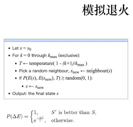
SA proposes a neighboring statefrom current state. For minimization, accept all improving moves; accept a worsening move with probability

At high temperature, the method explores and crosses barriers. Asdecreases, it becomes selective. The name reflects physical annealing, but the practical model is a nonhomogeneous Markov search over candidate solutions.

Cross the toy hill one move at a time

Start SA at, where the teaching objective is. Suppose its neighborhood proposes, where the objective is. The proposed change is, a worsening step. A greedy local method rejects it. At temperature, SA accepts it with probability. At, acceptance falls to. At, it is essentially zero. This is the whole point of temperature: early in the run, the method may cross a barrier to explore another basin; late in the run, it mostly refines what it has found.

If we do accept, a subsequent proposal tohas objective, an improvement ofover the current state. SA accepts an improving move without a temperature gamble. The sequencehas crossed from the right basin toward a better left basin. But accepting the uphill step is not enough if our neighborhood never proposes the next left step, and a single lucky sequence is not evidence of reliable performance. Run independent starts and record how often the search reaches a left-basin objective under the same evaluation budget.

What if the neighborhood can jump directly fromto? That move improves the objective and would be accepted immediately. But a distribution that proposes two-unit jumps may also miss fine local adjustments near a valley. A tiny-neighbor distribution can refine well but struggle to cross a wide barrier. The temperature schedule and proposal scale must be designed together. “Cool slowly” is not a cure for a neighborhood that cannot reach the useful region, just as a GA mutation rate cannot fix a chromosome that cannot represent a legal schedule.

We can derive an initial temperature from a desired acceptance probability instead of guessing. For a typical uphill move of size, suppose we want about half such moves accepted early. Solve, giving. If we wanted 80% acceptance,. These are not universal ideal temperatures; they are calibrated to the scale of this objective and proposed moves. If we multiply every objective value by 1000, the same physical move has, so temperature must scale accordingly to preserve the same acceptance probability. A temperature numeral has meaning only relative to the objective’s units.

At low temperature, SA behaves increasingly like a local improvement search. If the current state isand temperature reaches a value where crossing thebarrier is extraordinarily unlikely, the method may remain in the right basin. Cooling scheduledetermines how many evaluations happen while such barriers are still crossable. With, ten reductions multiply temperature by; with, ten reductions multiply it by about. The second schedule freezes much faster. But generation count is not evaluation count: if we make one move per temperature with the slow schedule and a hundred moves per temperature with the fast one, the comparison changes. State both the temperature sequence and proposals per level.

Keep current and best-found states separately. To cross the hill, SA may temporarily holdwith objective 1 even though it previously sawat 0.1. If the run ends before reaching the left basin and we return only the final current state, we could hand back a worse solution than one already observed. The best-found archive should remain at 0.1 until a better point arrives. The current state is for exploration; the best-found state is for reporting. This is SA’s version of the GA elite memory and the PSO personal/global memories, though the movement mechanism differs.

Neighborhood and cooling

The neighborhood determines what the algorithm can discover. For routing, use swap, insertion, and segment reversal. For a binary plan, flip one or several decisions. For real variables, perturb selected coordinates with a scale related to the current temperature.

A Boolean example from the lecture’s application list

The slide mentions Boolean satisfiability, often shortened to SAT. Let A, B, and C be yes-or-no variables. Consider the three clauses,, and. We want all three true. A candidate state is three bits. One simple objective for a heuristic is the number of clauses not satisfied; zero means we have found a solution. This is not a proof method for arbitrary SAT instances, but it gives a concrete score to a candidate assignment.

Try. The first clause is true because A is true. The second is false because bothand C are false. The third is true becauseis true. So this assignment has one unsatisfied clause. Flip only C from zero to one. The second clause becomes true, and the third remains true because B is still false. The objective drops from one to zero; an annealing search would accept that improving move at any positive temperature. For this three-bit example, enumeration of all eight assignments is simpler than SA. The point is that a “neighbor” has an unambiguous meaning—flip a bit and recompute the affected clauses.

In a large formula with many variables and clauses, a bit flip may satisfy some clauses while breaking others. Some local states have no single-bit improvement even though a satisfying assignment exists elsewhere. SA can sometimes accept a flip that increases unsatisfied count to cross such a barrier, provided its temperature and neighborhood allow later progress. But if the formula has a simple exact or specialized SAT solver, use that as a baseline or primary method. The existence of local traps is a reason to consider global or stochastic search, not a reason to ignore specialized solvers with strong guarantees.

Job-shop scheduling, another application named on the slide, needs a different neighborhood. A bit flip is unlikely to describe a legal shop schedule. One might swap adjacent operations on a machine, then decode the resulting order under job precedence and machine capacity. If a swap creates a cycle in precedence or delays a mandatory deadline, it is illegal or needs repair. Protein configurations require yet another state and physically meaningful move, with energy and geometric validity checked. SA supplies an accept/reject framework; the problem supplies the candidate structure and move set.

This is why the same temperature formula can appear in routing, SAT, scheduling, and molecular configuration while the algorithms are not identical in practice. For SAT,might be one extra unsatisfied clause; for routing, it is extra distance; for scheduling, it might be added makespan or lateness. A temperature of “one” has a different meaning in each objective unit. To transfer SA responsibly, transfer the logic of accepting a cost increase with a calibrated probability, then design and test the domain-specific neighborhood from scratch.

A geometric schedule is common:

Choose initial temperature so that a substantial fraction of moderate uphill moves are accepted. Cool slowly enough to explore, but define a fixed evaluation budget so that comparisons are fair.

The cooling rate is not a physical truth borrowed from metal processing. In this algorithm it is a control choice. Plot the fraction of proposed worse moves accepted at each temperature. If near zero at the start, the initial temperature may be too low or the proposed moves too large. If near one even at the end, the schedule may not cool enough to refine, or the proposed moves may be too tiny to reveal meaningful changes. Plot best-found objective beside acceptance rate so the reader can see whether exploratory moves led to new basins rather than only creating motion.

Now that both search stories are on the board, the useful question is not which metaphor sounds cooler. It is which representation, neighborhood, constraint treatment, and validation budget fit the problem we actually have.

Choosing between methods

Use PSO when variables are naturally continuous, parallel evaluation is useful, and information sharing is beneficial. Use SA when a meaningful neighborhood exists, especially for discrete configurations. Use neither merely because the objective is nonlinear: constrained local optimization or differential evolution may be more appropriate.

Match the candidate and movement rule

The depot case from lesson six is a natural question for PSO only after we specify the decisions. If depot coordinates are continuous and every proposed coordinate pair has a legally computed flow allocation, particles can share promising locations. If the company may choose only among five existing parcels, a discrete enumeration or facility-location MILP may be simpler and more exact. If each site’s shipment quantities are already fixed to one depot and we are locating a single facility, the weighted sum of Euclidean distances is convex in that facility’s coordinates; specialized convex or geometric-median methods may solve it more reliably than a stochastic swarm. “Distance appears in the objective” is not enough information to pick PSO.

Annealing is particularly natural when we can say what a nearby legal decision is. In the traveling-salesperson case, reversing a segment preserves all cities and changes a few edges. In a worker schedule, transferring one optional task between compatible workers can be a local move if travel and overlap are rechecked. In a discrete facility configuration, opening one parcel and closing another may be a local move if capacity still covers demand. Without such an interpretable neighborhood, an SA temperature formula cannot create a meaningful search. We have to design the moves before choosing the cooling rate.

PSO can also be used on continuous parameters of a simulation, such as the weights of a patient-priority rule, but the objective evaluation then has noise and may be expensive. SA can search discrete staffing by moving one worker between shifts. The next workshop uses an emergency-department queue to see those choices in context. The methods’ parallel versus single-trajectory character affects runtime, but feasibility, decision timing, and fair comparison still come first. A method is appropriate when its representation and movement exploit the decision’s structure, not when its name sounds suitable for “global optimization.”

Experimental protocol

For stochastic optimization:

• fix and report multiple random seeds;
• compare under equal objective-evaluation budgets;
• plot median and quantiles across runs;
• record feasibility rate and runtime;
• verify the best returned solution independently;
• benchmark small instances against an exact method.

Stopping because “the curve looks flat” is not reproducible. Use a maximum evaluation count, time limit, or no-improvement window, and report it.

Global search finds candidates; it does not replace modeling. The final paper must still justify variables, constraints, objective, uncertainty, and validation.

What should the comparison plot actually show?

On our toy, we can evaluate a dense grid or use a reliable local solver from multiple starts to understand the left and right basins. The grid is an oracle for the teaching example, not a method we can always afford for a high-dimensional simulation. Run PSO and SA many times from independently drawn legal starts, with the same number of objective calls per run. For each call, record the best feasible objective seen so far. Put evaluation count on the horizontal axis, not PSO iteration on one curve and SA temperature level on the other. Otherwise the two curves silently use different amounts of work.

Show individual thin curves or a median curve with a spread band. If most PSO runs reach the left basin quickly but a few collapse in the right basin, the median alone might look strong while the failure rate matters to a risk-averse decision maker. If SA sometimes crosses the hill late, a fixed early cutoff might miss that behavior. Record the fraction of runs whose best value falls below a declared left-basin threshold and the evaluation count at which they first do so. Do not choose that threshold after seeing one method’s outcomes; derive it from the known toy landscape or a predeclared quality standard.

Feasibility belongs on the same dashboard. A depot swarm may report low cost at illegal river coordinates; a route annealer may report short travel time with a capacity violation. Count legal candidates, maximum violation, and how often repair changes an objective. The “best objective” curve must be best legal objective. A method that creates many beautiful illegal points may have useful exploratory information, but it has not produced a company decision until one of them is repaired and independently checked.

Runtime can differ even with equal objective calls. PSO can evaluate particles in parallel when each evaluation is independent. SA’s current state depends on preceding accept/reject decisions, so its main chain is sequential, though independent chains can run in parallel. If the depot candidate evaluation itself solves an LP, that cost may dominate movement arithmetic. If the emergency-department candidate evaluation runs twenty simulation replications, that cost dominates too. Report both calls and elapsed time on the actual hardware, without attributing a faster implementation to a better mathematical search rule.

Tune parameters on separate pilot cases, then freeze them for final comparison. For PSO, test inertia, attraction coefficients, swarm size, and boundary handling. For SA, test proposal scale, initial acceptance rate, cooling, and moves per temperature. If we tune all of them on the final test problem until one method wins, the comparison has overfit the instance. Use several representative instances and show whether a chosen configuration is reasonably stable across them. A competition report can be concise about this process, but it should not hide the fact that parameter tuning used computational budget and data.

There is another honest competitor: a deterministic or quasi-deterministic solver matched to the structure. SciPy’s official optimization guide lists bounded global-search alternatives and their supported constraints (guide ). A continuous differentiable depot subproblem may not need a swarm; a route can be improved by 2-opt; a small SAT or scheduling instance can be enumerated. We should not compare PSO only with SA and declare both useful. Compare with the strongest simple structure-aware method that fits the task and deadline.

Finally, independently recompute the returned decision’s objective and rules. If a proposed depot is at, list its coordinates, legal-site status, allocated shipments, each site’s demand balance, each depot’s capacity, and total ton-distance. If a staffing policy is chosen, translate search coordinates into worker counts or priority thresholds, rerun held-out scenarios, and show wait and overtime together. The plot demonstrates a search process; the decision audit demonstrates that a physical recommendation exists. Both are needed.

Implementation skeletons

For PSO, initialize bounded positions and modest velocities, then update personal and global bests only after evaluating repaired candidates:

initialize x, v, personal_best
global_best <- best(personal_best)
repeat:
    v <- inertia*v + cognitive*rand()*(personal_best-x)
         + social*rand()*(global_best-x)
    x <- enforce_bounds(x+v)
    evaluate x
    update personal_best and global_best

For SA, keep the best state separately from the current state. The current state may worsen temporarily, while the best state should never be forgotten.

current <- feasible_initial_state()
best <- current
for temperature in cooling_schedule:
    repeat moves_per_temperature times:
        candidate <- neighbor(current)
        delta <- cost(candidate) - cost(current)
        if delta <= 0 or random() < exp(-delta/temperature):
            current <- candidate
        if cost(current) < cost(best): best <- current

Plot acceptance rate by temperature. If it begins near zero, the initial temperature is too low or moves are too large; if it remains near one, cooling is too slow or moves are too small.

The fixed-compute question in the slide

The lecture’s annealing application slide points to a practical tension: when computation is limited, a good approximate global candidate may be more useful than spending the whole budget polishing one local basin to extreme numerical precision. We can put numbers on that budget. Suppose one objective evaluation is a depot LP solve or a clinic simulation. A PSO run with ten initial particles and one hundred rounds producing ten new evaluations each uses aboutobjective evaluations. An SA run allowed 1010 evaluated neighbor proposals gets the same number of objective calls. The outer arithmetic of both methods is cheap compared with the depot or clinic evaluator.

If each clinic-policy evaluation itself averages twenty simulated days, those 1010 calls represent 20,200 clinic-day runs per optimizer seed. Thirty independent seeds would represent 606,000 clinic-day runs before final held-out validation. That may be far too costly. We could reduce candidate calls, use a smaller but paired scenario set during search, build a justified surrogate, or reserve most replications for the finalists. But whatever economizing we do should be applied fairly and reported. A chart showing “100 PSO iterations versus 100 annealing temperatures” without counting the inner simulations would miss the true resource constraint.

What does “approximate global” mean here? Neither PSO nor ordinary practical SA proves that a returned clinic policy or depot location is globally optimal under a finite run. We can say it searched broadly across starts or configurations and found a candidate better than a legal baseline under the measured budget. If an exact small instance or valid bound exists, compute a gap there. If no bound exists, report best-found objective, variation across seeds, and sensitivity to starting points. A local solver returning eight decimals at one basin may be less useful than a broad search finding a much better basin, but a broad search’s best value is still a measured candidate, not a guarantee.

Parallelism changes wall-clock feasibility. Ten PSO particle evaluations can often run simultaneously, though a shared global-best update still requires synchronization after those evaluations. One SA chain’s next proposal depends on whether the previous one was accepted, so that chain is sequential; multiple independent chains can be run in parallel and compared. On one laptop, parallelism may be limited by memory or simulator overhead. On a cluster, it may substantially shorten PSO wall time. Report hardware and whether method calls were parallel rather than attributing every time difference to better search logic.

The fixed budget also shapes stopping and reporting. If a method is stopped at 1010 calls, preserve the best legal state found even if its current state is worse. Show the curve at call 1010 and perhaps at earlier call 250 and 500 to reveal whether the recommendation depends on nearly the full budget. If the leading candidate changes after a small change in random seed or objective data, its operational confidence should be limited. The slide’s point is not “metaheuristics always beat exact local search.” It is that, under finite resources, we must decide what kind of accuracy and guarantee matters for the decision, then spend and report the budget accordingly.

Search, simulation, and a queue

Metaheuristics are often used around a simulation whose output has no simple formula. Suppose an emergency department chooses staffing levels and patient-priority rules. The objective combines waiting time, overtime, and the fraction of high-severity patients served late. A discrete-event simulation estimates these outcomes for one candidate policy.

Build a discrete-event simulation

The simulation state contains the clock, waiting queues, busy servers, and patient records. Events include arrival, service start, and service completion. The basic loop is:

1. remove the earliest event from a priority queue;
2. advance the clock to that event time;
3. update state and statistics;
4. schedule any events caused by the update;
5. stop after the warm-up and observation horizon.

Do not advance time in tiny fixed increments when nothing happens. Event-driven simulation is both faster and conceptually clearer.

Watch three patients pass through one desk

Suppose patient 1 arrives when the clinic clock reads 0 hours and needs 0.15 hours of service. Patient 2 arrives at 0.10 hours and also needs 0.15 hours. Patient 3 arrives at 0.20 hours with the same service requirement. There is one server, first-come-first-served, no break, and no preemption. Patient 1 starts immediately and completes at 0.15 hours. Patient 2 has already arrived at 0.10, so they wait until 0.15, then finish at 0.30. Patient 3 arrived at 0.20 and waits until 0.30, then finishes at 0.45. The waiting times before service are,, andhours. Their average ishours, or three minutes. This little queue is not anrandom sample we are using to estimate long-run formulas; it is a fixed hand-checkable event trace.

Write the event table to make the simulation rule visible:

Patient	Arrival (h)	Service start (h)	Completion (h)	Queue wait (h)
1	0.00	0.00	0.15	0.00
2	0.10	0.15	0.30	0.05
3	0.20	0.30	0.45	0.10

At time 0.10, the queue contains patient 2 and the server is still busy with patient 1. At 0.15, patient 1 completes and patient 2 starts; the simulator does not need to tick through every thousandth of an hour between those events. At 0.20, patient 3 joins the queue. At 0.30, patient 2 completes and patient 3 starts. If code reports patient 3 started at 0.20 while there is only one server, it has a capacity bug. If it reports a negative wait, it may have sorted events or updated the clock incorrectly. A small fixed trace can test an event simulator before random arrivals and realistic priority rules are added.

Now ask a staffing question rather than simulating for its own sake. A manager could add a second server during the busy 0.10–0.30 interval. Patient 2 might then start on arrival at 0.10, while patient 3’s start depends on when that second server finishes and whether the first is free. The additional staff-hours cost money; the queue waits change. The simulator must report both waiting outcomes and staffing cost under the same arrival trace. An optimizer cannot decide whether a second server is worth adding until the decision maker tells us whose waiting matters, what the cost is, and whether any patient has a maximum acceptable delay.

The patient-priority rule is another decision. If patient 3 is critically ill, first-come-first-served might be inappropriate; we may allow them to jump ahead at the next service completion. But do not accidentally preempt an ongoing medical procedure if the real desk cannot interrupt it. Priority changes the state and event logic, not just a weight in a formula. A credible model names whether service is preemptive, how severity is known at arrival, and whether shorter waits for high-severity patients cause longer waits for others. Only then does a priority weight become a meaningful continuous parameter for PSO.

For a simplequeue with Poisson arrival rateand exponential service rate, utilization is. When,

and Little’s law gives. Use these formulas to verify a simulation before adding priorities, multiple servers, or empirical distributions. Whenapproaches one, delay grows nonlinearly; average capacity being barely above average demand is not enough.

Why eighty-percent utilization can still mean a long wait

Take arrival ratepatients per hour and service ratepatients per hour for a single idealized server. Utilization is. If arrivals really are Poisson, service times exponential and independent, the system reaches a stable long-run regime because. The formula above gives mean time in the system, including service,hours, or thirty minutes. Average service time alone ishour, six minutes, so mean waiting before service is twenty-four minutes. The average number of patients in the whole system is; the average number waiting, excluding the one in service on average, isunder the same model.

If arrivals rise to nine per hour while the same server still handles ten per hour, utilization becomes 0.9. Mean time in system jumps tohour: sixty minutes, of which roughly six are service and fifty-four are queue wait. If arrivals reach 9.5 per hour, utilization 0.95 andhours. The system has spare capacity of only half a patient per hour; random arrivals can build a backlog faster than it drains. This is why “average capacity is just above average demand” is a weak service recommendation. Near the stability boundary, a small input change can have a large delay consequence.

Do not apply the thirty-minute number to a real emergency department without checking assumptions. Severe patients may get priority, service times may be heavy-tailed or depend on severity, there are multiple clinicians and rooms, arrivals vary by hour, and some patients leave before service. Theformula is a verification benchmark for a deliberately simplified simulator: when we turn off priorities and feed it Poisson arrivals and exponential service with rates 8 and 10, its long-run estimates should approach the theoretical values within simulation uncertainty. If they do not, we investigate event ordering, warm-up, service-time generation, and metric definitions before optimizing staffing.

Little’s lawis also an accounting check under stable conditions and consistent boundaries. Ifmeans total time in the system,must count patients waiting and in service. Ifmeans waiting before service, compare it with, the queue-only count. Mixing those definitions can make a correct simulator appear wrong or a wrong one appear correct. The hand trace above used queue wait, whereas theformula first gave total system time. State which one the manager’s objective actually values.

If utilization reaches or exceeds one in the continuing idealizedqueue, the stated stationary formulas do not apply; backlog tends to grow rather than settle to a finite long-run mean. A single clinic day may still end or close, leaving people unserved, but that is a different terminating-system question. The distinction matters: a formula’s denominator approaching zero is not a software error we can patch with a tiny constant. It is a warning that the assumed long-run operating regime breaks down.

Understand Markov structure

If the future state depends on the present state but not the full past, transitions can be written in a matrixwith. A distribution evolves as. A stationary distribution satisfiesand. Markov chains model weather regimes, customer states, reliability, and inventory conditions, but the memoryless assumption must be tested or justified.

A two-state weather clock

Think of weather as either Clear or Storm. In a toy daily transition model, a clear day is followed by another clear day with probability 0.8 and by a storm with probability 0.2. A storm is followed by clear weather with probability 0.4 and another storm with probability 0.6. Put current states in rows and next-day states in columns:

Every row sums to one, because from each current state tomorrow must be one of the two states. If today is certainly clear, the state distribution is. Multiplying once gives. Multiplying again gives. The storm probability two days from now is 0.28, not 0.2, because tomorrow might already be a storm and storms have a 0.6 chance of persisting. A model that draws each day’s weather independently with storm probability 0.2 would miss that persistence.

The stationary distribution in this toy balances clear-to-storm flow against storm-to-clear flow. Letand require. We obtainand. If the transition probabilities remain fixed for a long time and the chain’s usual mixing conditions hold, the daily state distribution approaches that balance. This does not mean exactly one in every three consecutive days is a storm, nor does it make the next-day forecast independent of today’s state. It is a long-run probability under the toy transition mechanism.

Why include a weather chain in a search-method lesson? Suppose storm days raise clinic arrivals. Staffing chosen for a sequence of days should account for storms that cluster, not just for a single average arrival rate. A simulation can draw daily regimes from, then draw patient arrivals conditional on regime. The decision maker might change staffing after today’s observed weather or before tomorrow’s weather is known. That decision time defines what information the policy may use. PSO or SA can tune a policy’s parameters, but the regime process belongs in the simulator and must be validated separately.

The Markov assumption is strong: tomorrow depends on today’s category but not directly on the prior week after today’s state is known. Real weather, outbreaks, customer loyalty, or equipment reliability may remember duration, season, and hidden conditions. Check whether observed transition frequencies change by season or by how long the system has stayed in one state. If they do, add duration or season to the state, use a more suitable model, or avoid claiming a Markov chain captures the full mechanism. A neatmatrix is a teaching device until data support its memory assumption.

Optimize noisy outputs

One simulated objective value is noisy. Compare policies using common random numbers: run competing candidates on the same arrival and service scenarios so that differences have lower variance. Use multiple replications and optimize an estimated mean plus risk term. Cache evaluations when the same discrete policy returns.

A policy score is a measurement, not a fact

Suppose staffing policy A and policy B are evaluated on one simulated clinic day each. A happens to see twelve arriving patients and B sees twenty. Even if B has more staff and a better priority rule, B may report a larger average wait simply because its simulated day was busier. Comparing those raw outputs would confuse the policy effect with arrival randomness. Generate one arrival and service-time scenario, then run both policies on that same scenario. Repeat across many independently generated scenarios. For each scenario, compute B minus A in the manager’s outcome. The paired differences show whether B typically improves wait under comparable conditions.

For the three-patient fixed trace above, both policies should receive arrivals athours and the same service requirements. If one policy adds a second server, its change in queue wait is attributable to that staffing rule in the trace, not to a different draw of arrivals. On a realistic simulation, we use many such matched traces and report variability. If the manager cares about critically ill patients, record their waiting distribution separately rather than hiding them inside an average across all severities. A policy that reduces mean wait while making a few critical waits dangerously long is not automatically an improvement.

Now define a policy objective carefully. We might use expected total waiting minutes plus a declared cost per extra staff-hour and a much larger cost for critical-patient lateness. But if lateness beyond a clinical limit is prohibited, model it as a constraint or a separate safety outcome, not merely a price that the optimizer can pay. If the manager says, “No critical patient may wait more than ten minutes in the modeled stress scenarios,” that is a feasibility rule. If they say, “We strongly prefer shorter waits but cannot add unlimited staff,” that is a trade-off. Exactly as in our factory goal example, the words cannot and prefer lead to different mathematics.

PSO might tune continuous policy thresholds or priority weights. One particle is a vector of such settings, and one evaluation runs multiple clinic-day simulations under those settings. SA might move one worker from a quiet afternoon shift into a busier evening shift, giving a neighboring discrete staffing plan. If we use PSO for integer worker counts by simply rounding every particle coordinate, many distinct particle positions decode to the same staffing plan and velocities become hard to interpret. A discrete SA neighborhood or a mixed-integer staffing model may be cleaner. Again, the choice follows the decision’s type, not the optimizer’s reputation.

Suppose an optimizer evaluates fifty policy candidates, each on ten simulated days. That is roughly 500 clinic-day simulation runs, even if its outer plot shows only fifty dots. If one candidate uses a more expensive simulator version or gets twenty days of evaluation, budgets are not comparable. Count simulation replications as the costly unit. Keep a separate held-out scenario set for the finalists; otherwise a search that repeatedly uses the same ten scenarios can learn their accidental details. We saw this overfitting issue with GA parameter search, and it persists for PSO and SA.

If the simulation is noisy, PSO’s personal-best and global-best memories can preserve a lucky low score for too long. A particle might be marked “best” because it happened to encounter an unusually quiet day. Periodically re-evaluate promising memories with additional matched replications, or use confidence-aware comparisons before replacing a current best. SA’s acceptance rule has the same issue: an apparent objective differencemay be simulation noise rather than a real policy change. Use enough replications to estimate it, and make clear whether the temperature is calibrated to true policy-cost differences or noisy one-day outputs. Search mathematics cannot turn an unreliable evaluator into reliable evidence.

The final recommendation should include an operational rule: which shift receives additional staff, under which arrival forecasts or severity mix, how much overtime is expected, and what stress scenario would cause the policy to be reconsidered. “PSO converged at” is not useful until those coordinates are decoded into actual clinical decisions. The queue simulation, search method, and reporting layer form one chain. A mistake in the first link can make every later decimal impressive but irrelevant.

PSO is natural for continuous parameters such as priority weights; SA is natural when a policy has a meaningful local move, such as transferring one worker between periods. A hybrid can use PSO or SA globally and a deterministic local search for refinement. State the total simulation replications because they dominate computational cost.

Remove initialization bias

For a continuing queue, an empty system at time zero is unrepresentative. Plot time-series averages and discard a justified warm-up period, or initialize from an approximate steady state. For terminating systems such as one clinic day, the empty opening state may be real and should not be removed.

Why the first simulated minutes can lie

If we simulate a clinic that operates continuously day and night but initialize it with zero waiting patients and an idle doctor at time zero, the first arrivals are likely to receive unusually fast service. The long-runexample atpredicts total time around thirty minutes, yet a short simulation starting from emptiness could report much less simply because it has not built the ordinary queue. That is initialization bias. A warm-up period discards early measurements after the system has begun to resemble its continuing regime, while still allowing its early events to influence later state. We should inspect running averages or queue-length traces and justify where measurement begins, not choose a cutoff solely because it makes a favored staffing policy look better.

Now consider a clinic that actually opens at 8:00 a.m. with an empty waiting room and closes at 5:00 p.m. Its opening emptiness is a real feature, not an artifact. Discarding the first hour would hide a genuine part of the daily experience. This is a terminating simulation of a day, and we should compare complete days under matched arrivals. The right warm-up treatment follows the physical system boundary. It is not an optional software preference.

Different staffing policies can change how quickly a queue builds. If we run policy A and B with the same continuous arrivals but remove a warm-up period of unequal length chosen after seeing their curves, we bias the comparison. Choose the measurement rule in advance and apply it consistently, or initialize both from comparable steady-state conditions. For a full-day clinic, compare from opening to closing and report any carryover patients or overtime after closing. A policy that clears its queue only by working two extra hours needs that cost and patient experience included.

Independent replications are also important. One long stochastic run contains many patient observations, but their waits are dependent through the shared queue state. Treating every patient as an independent trial can make uncertainty bands unrealistically narrow. Run many independently generated days or continuing-system replications, calculate each replication’s policy metric, and summarize the distribution across replications. With paired common random numbers, compare policy differences within each replication. A confidence interval for the policy difference is more directly useful than two unrelated confidence intervals for their separate means.

If severity groups differ, report subgroup results. Mean wait could drop because many low-severity patients wait less while a small critical group waits more. State how severity is measured at arrival, whether priority can change after triage, and which threshold defines “served late.” The simulation should preserve these operational meanings before optimization begins. PSO may tune a numeric priority weight, but the weight is only a policy coordinate; the clinically meaningful result is the distribution of who gets served when under that policy.

We have now connected event simulation back to search. A search method can propose many staffing or priority candidates. The simulator converts each into an estimated outcome. The warm-up, scenario set, metric definitions, and replication count determine how trustworthy that estimate is. If those upstream pieces change, the optimizer’s favorite candidate may change too. A well-written article therefore treats the simulator as part of the model, not as a silent box behind the optimizer.

Practice

Simulate anqueue and verify Little’s law over severalvalues. Replace exponential service with a two-component empirical mixture and observe the tail. Then choose staffing for each period using SA, with common random numbers and a penalty for late high-severity patients. Report confidence intervals and compare with a rule based only on average utilization.

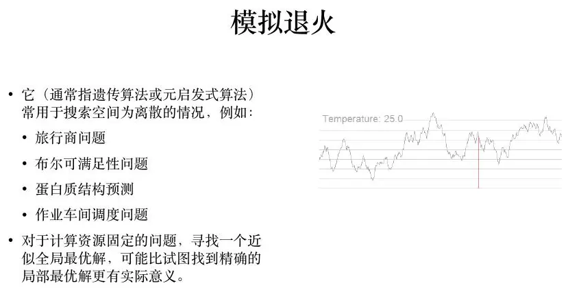
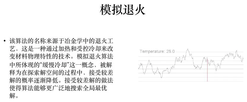
The workshop made the methods concrete on a small problem. Returning to the lecture figures will show how their trajectories and acceptance rules are usually drawn—and which parts a figure must label to be interpretable.

PSO and annealing as shown in the course

Each particle carries position and velocity through a shared landscape.

Personal and global best are memories, not current positions.

Implementation must expose boundary handling and stopping.

Social sharing accelerates consensus; cognitive memory protects exploration.

Routing, SAT, protein configurations, and job shops require problem-specific moves.

Controlled cooling reduces acceptance of worse states gradually.

Acceptance connects objective increase and temperature.

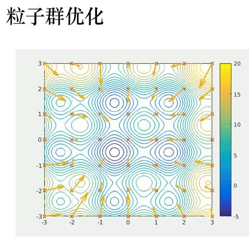
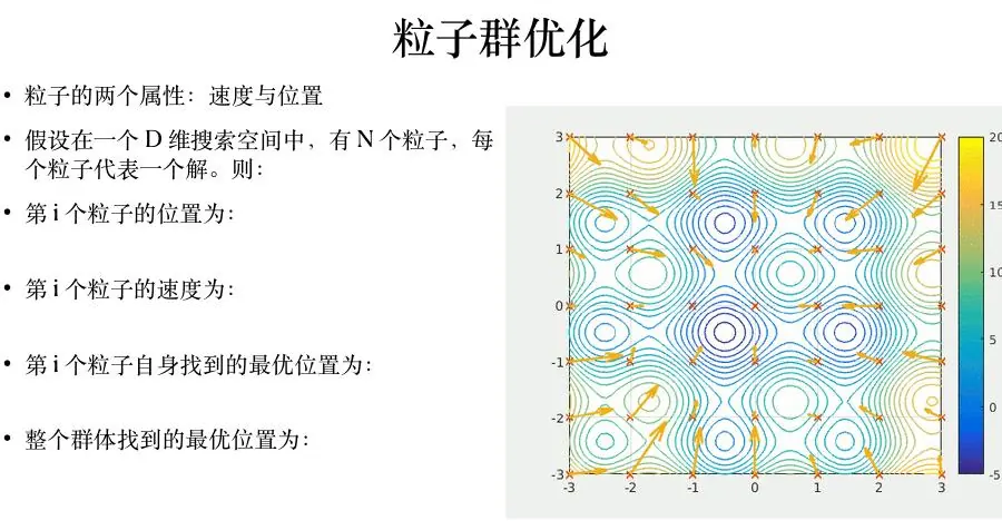
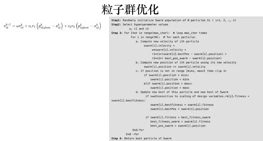
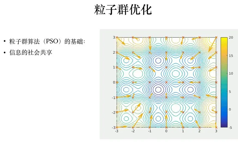
For particle,

is personal best,swarm best. Largesustains motion; smalldamps it. Velocity clipping prevents explosion but changes geometry. Reflection usually preserves more search information than blunt coordinate clipping.

Annealing accepts improvements and accepts deteriorationwith

Chooseso typical uphill moves have a planned acceptance rate. Routing uses swap, insertion, or 2-opt; scheduling uses feasibility-preserving moves or repair. Cooling without a suitable neighborhood cannot rescue the search.

Return to the six-site cement map

The six construction sites from lesson six make a useful final decision story. Their daily demands add to 36 tons, and the two existing depots atandeach have 20 tons available. Under the stated Euclidean ton-distance measure, the feasible fixed-depot shipment plan costs aboutdistance-weighted ton units. That number is a baseline for transport under existing locations, not a bill in yuan unless a price per ton-distance is supplied. The nearest-depot map with cost aboutis infeasible because B would ship 21 tons; it cannot be used as the comparison policy.

Suppose the company is allowed to relocate the depots anywhere within two legal parcels or coordinate regions. A PSO particle could store candidate coordinates for both depots. For every particle, solve the fixed-coordinate transportation LP to allocate 36 tons legally and return its best transport objective. This keeps the capacity and demand accounting exact inside each candidate evaluation. The PSO outer search then explores the nonconvex location question. Its reported “best found” coordinates should be accompanied by the positive-flow routes, shipment quantities, total cost, parcel legality, and comparison with the existing-depot baseline. A particle with low distance but no legal shipment allocation is not a viable improvement.

If instead there are only five approved parcel sites, a continuous coordinate swarm is awkward: most particle positions are not approved parcels. We could encode a pair of parcel indices, enumerate the ten unordered pairs, and solve a transportation LP for each. Ten exact comparisons are simpler and more auditable than a swarm. For fifty or five hundred parcels, discrete facility-location optimization or an SA neighborhood that swaps one selected parcel may be reasonable. The mathematical class changes when we replace “any coordinate” with “choose approved parcels.” The earlier lesson’s warning about variable definitions still decides which method makes sense.

Consider one SA move in that discrete case. Current state selects parcels P and Q; the neighbor replaces Q with R while keeping P. Decode the pair, solve its legal shipment allocation, and calculate the change in transport cost plus any relocation or site-opening cost. If the new pair is worse by 100 cost units, a high temperature may sometimes accept it to explore configurations reachable beyond R; a low temperature usually rejects it. But “100” may mean ton-distance, yuan, or a mixed score. The temperature has to use the actual objective units. The neighbor rule must also prevent choosing the same parcel twice if two distinct depots are required.

What if construction cost dominates transport saving? Suppose the search reduces ton-distance by ten units but moving depots costs hundreds of thousands of yuan. We cannot declare relocation worthwhile from the transport measure alone. Convert ton-distance to actual operating cost over a stated horizon, add construction and inventory-transfer costs, and compare net value. If the course exercise intentionally minimizes only transport work, report that narrower answer honestly and say the economic recommendation requires additional terms. An algorithm cannot optimize an expense we never wrote down.

Demand uncertainty matters too. Site 6 currently needs eleven tons; if its demand rises, a location that looked good under the original 36-ton total may require a different flow or become capacity-tight. Re-evaluate leading coordinate pairs under several plausible demand vectors. A map of recommendation stability can show which parcels remain favored and which routes are fragile. PSO and SA find candidate locations under a nominal model; scenario checks tell us whether those locations are robust enough for a real decision. Keep the candidate-search data separate from the held-out or stress cases used to assess the recommendation.

This depot story is a fair test of our method-choice understanding. Fixed locations yield an LP. A small finite parcel list yields enumeration. A large parcel choice suggests discrete optimization or SA-style neighbors. Continuous joint location and flow can invite an outer search such as PSO around an inner LP. The same six-site data support all four formulations because the question changes. The lesson is not “use PSO for depots.” It is “state the decisions and guarantees, then select a search method appropriate to the resulting structure.”

From a search point back to a person

The emergency-department example gives the same reporting challenge with human consequences. A PSO vector of priority thresholds or an SA staffing configuration is not a result a chief nurse can implement from a graph alone. Translate it into shift staffing, triage rule, expected total wait, high-severity wait distribution, overtime, and the arrival scenarios used to estimate those outcomes. Compare with current staffing and a simple surge rule under matched simulated days. Check that the chosen rule is feasible under the minimum staffing and break requirements. Then stress a sudden high-severity cluster or one absent clinician. The “best found” simulation score is only one line in that report.

An action statement might read: “For morning arrival patterns resembling the tested exam-week scenarios, add one triage clinician during the observed peak and use the declared severity-first rule; re-evaluate if the critical-patient arrival rate exceeds the tested range.” We cannot fill that statement with measured times or confidence intervals without actual clinic data, so it remains a model of what evidence a real study would need, not a fabricated result. The wording is useful because it names the action, setting, trigger, and limitation. If a particular simulated policy wins only because one noisy day was unusually quiet, the paired replication analysis should prevent us from presenting it that way.

We should also ask whose loss the objective hides. A mean wait can decrease while the tail for an important subgroup increases. A staffing cost can fall while a clinician’s overtime becomes unsafe. The manager’s priorities should be visible as hard constraints, separate outcome columns, or approved weights. We learned that in the multiobjective lesson; global search does not erase it. A plot of optimizer convergence cannot reveal ethical or operational trade-offs that were absent from the evaluator.

Finally, use a small counterexample to challenge each reported winner. For a depot, check a one-ton demand perturbation that forces capacity reallocation. For a route, check a time-window boundary. For a clinic, check the fixed three-patient trace before any stochastic experiment. These examples are the specific failure points suggested by the particular model. Their job is to make a claim falsifiable. When a search output survives them and a fair baseline, we can speak about its usefulness with an appropriate, limited confidence.

Search methods choose among candidate decisions; dynamic models describe how a system evolves after a decision or initial state. The next lesson therefore changes our central question from “Which point is best?” to “How does the state change over time?”
Search methods choose among candidate decisions; dynamic models describe how a system evolves after a decision or initial state. The next lesson therefore changes our central question from “Which point is best?” to “How does the state change over time?”

We have already met that second question inside the search examples. A clinic staffing vector is one decision, but patient arrivals, queues, and server availability evolve event by event after the shift starts. A depot coordinate is one decision, but daily site demand can change after the warehouse is built. A route order is one decision, but arrival time accumulates along each edge and changes whether later appointments remain feasible. PSO and SA move candidate decisions around; they do not by themselves provide the clock and state laws that determine a candidate’s score. The evaluator must contain those laws.

Return briefly to the hot-water basin from our first lesson. The basin starts atand must remain at or above an illustrativethreshold after each plate batch. Suppose, for a deliberately simple hand check, the water has heat capacitykJ per degree Celsius and each batch removeskJ. With the heater off and no room loss, each batch lowers temperature by. The temperatures after successive batches are. Only the first two remain above the threshold; the third does not. We did not obtain that result by searching an objective landscape. We obtained it by updating the state from one batch to the next under an energy rule.

Now suppose the heater supplieskJ during each batch. The net energy loss iskJ, so the toy temperature falls byper batch. The sequence after five batches is; a sixth would fall to. Heater use raises the modeled number of acceptable batches from two to five. But energy is not free, and the simple constant-20-kJ plate removal may fail as plates or water temperatures change. The original basin model should be validated before an optimizer recommends a heater policy. If the tiny state calculation is wrong, a global optimizer can only find the best decision for a wrong process.

Suppose we may choose heater inputfor each batch, under a total energy budget. One candidate policy is a sequence, and its evaluator repeatedly updates basin temperature, checks the threshold after every batch, and counts the plates or energy cost. This is an optimization around a dynamic model. For three or five batches, enumeration or dynamic programming may be clearer than PSO or SA. For a complicated basin with uncertain room loss, nonlinear heat transfer, and many control choices, a global or stochastic search could be useful—but only after the state law and constraints are defined. The method does not create energy conservation; it searches decisions evaluated through that conservation law.

This explains the difference between a search trajectory and a physical trajectory. The path of a PSO particle across coordinate space is not a truck’s daily route or a robot’s motion over time; it is the algorithm’s exploration of proposed decisions. SA’s temperature is an acceptance-control parameter, not necessarily the physical water temperature in a basin or a furnace. The same word “temperature” can describe a real thermal state and a search parameter with completely different meanings. Keeping those meanings separate prevents a beginner from confusing an optimization metaphor with the system being modeled.

The next chapter will derive rate laws for physical state variables—position, angle, fluid height, and temperature—rather than update rules for optimizer candidates. We will ask what quantity accumulates, what flow or force changes it, what initial or boundary condition is known, and what observation could show the law is too simple. After we understand a state equation, we can return to optimization and ask which control or starting choice produces a better outcome. The order matters: first make the dynamics credible, then search over decisions that depend on them.

The heater result has almost no safety margin at the fifth batch: it lands exactly at. If each batch removeskJ rather thanwhile the heater still supplies, net loss iskJ and temperature fallsper batch. The first three batches end at; the fourth ends atand fails. A five-batch recommendation based on the nominal 20-kJ estimate would not survive that plausible perturbation. This is a dynamic sensitivity test with an operational implication: measure plate heat demand or leave a temperature reserve before scheduling five batches. A particle cloud or annealing trace cannot substitute for that check.

There is also a decision-time distinction. If the operator can read a thermometer after every batch and adjust heater input before the next, a feedback policy maps observed temperature to action. If the heater schedule must be programmed in advance and cannot be changed during washing, the decision is a fixed input sequence under uncertainty. Those are different candidate objects for an optimizer. They also demand different evidence: a feedback rule depends on sensor accuracy and response delay, while a fixed sequence depends more heavily on worst-case plate and room-loss assumptions. We will learn to express changing state and input explicitly in the next lesson.

Think of the clinic in the same way. A fixed number of nurses chosen before patients arrive is a schedule; a surge rule that adds staff after a queue-length alarm is feedback. PSO or SA can search parameters of either policy, but the simulator must know what information is available at each time and how the queue changes after an action. The physical or human process is the substance; the search method is a way to choose among well-defined controls.

If the queue-length alarm is set at five waiting patients, the feedback policy also needs a response time: can another nurse arrive immediately, ten minutes later, or only next shift? An optimizer might set the threshold beautifully, but the benefit disappears if the extra worker arrives after the busy period. Test the same arrival trace with the true response delay. For the basin, the heater likewise cannot add ten kilojoules instantly if it takes a minute to warm up. Dynamic constraints turn plausible controls into actual controls. A global search over impossible instantaneous responses would be impressively precise and operationally wrong.

That is the final connection between today’s algorithms and tomorrow’s equations. PSO and annealing can compare candidate locations, settings, or policies, but an evaluator must follow a system from one state to the next under the chosen action. In the static cement map, flow allocation is the inner model; in the clinic, event updates are the inner model; in the basin, energy balance is the inner model. The outer search cannot be stronger than the inner description. When a result changes under a small state-law correction, repair the description before spending more evaluations on an old optimum.

Before lengthening a search run, ask whether a better candidate would matter to the real decision and whether the evaluator’s main assumptions have survived basic checks. If not, invest the next stage of work in measurement, validation, or a better state model. A longer trace is valuable only when the score it explores has meaning. The bottleneck is often our description of reality, not the number of optimizer updates. If a tiny event trace fails or a depot shipment violates capacity, fix that failure before presenting any curve as evidence of a better decision.