Search algorithms choose among candidate answers, but some modeling questions ask how a system changes while time passes. Imagine a water tank with a hole in its side. The water level falls quickly at first and more slowly later. How could you predict when it reaches the mark where a pump must turn on? We need a quantity that changes, a rule for its rate of change, and its starting value. That is the basic story of a differential equation.
We will practice the story on a pendulum, a pursuit path, a draining vessel, and heat conduction. In every case I will ask you to describe what is stored or moving before displaying the derivative. You should be able to test a sign, unit, and limiting case, then decide whether a numerical solution is necessary. The pictures in the slide deck are not decorations: each should help you identify the state and the physical mechanism.
Differential equations model mechanisms expressed as rates. The central question is not “which ODE should I memorize?” but “what balance or law determines the derivative of each state?”
State, rate, and initial condition
Choose the smallest state vectorthat makes the future determined by the present and inputs. Then write
Parametershave units and sources. Initial conditions are part of the model; without them, an evolution law does not specify one trajectory.
Higher-order equations can be rewritten as first-order systems. If, letand, givingand.
Begin with a measurement a student could make
Put a ruler against the tank from the opening question. At noon the water depth is one metre; a minute later it is lower. We could describe the fall by an average difference,, measured in metres per second. A derivativeis the limiting local version of that ratio: how fast the level is changing at the current depth. We use it because the outflow speed itself depends on depth. A single “the tank loses two centimetres per minute” rate may be reasonable for a short interval but will not stay constant all the way to empty.
The state is what we need to carry from now to later. For a simple tank with a known cross-sectional area and a hole, water depthmay suffice. For a heater-controlled basin, we might also need water temperature and heater state. For a moving patrol craft, we need position and perhaps heading. A state is not every variable in a spreadsheet; it is the minimal information that, together with inputs and parameters, lets the model determine its next change. If hidden memory matters—such as a heater that warms up slowly—then “current water temperature only” is not enough and the state must grow.
An initial condition pins the story to one actual experiment. The lawdescribes many possible draining trajectories: a tank starting at one metre, another at half a metre, and another at two. Sayingmetre selects the first. If we start a pendulum from a specified angle, we must also state its initial angular velocity because its equation is second order. If we prescribe rod temperature at both ends for a steady spatial ODE, those are boundary conditions rather than an initial time state. We cannot repair missing conditions by lowering a numerical tolerance; the model has not yet identified a unique physical solution.
A cylindrical tank as the simplest conservation law
Before the hemisphere in the slides, consider a cylinder with horizontal water area, outlet area, discharge coefficient, and starting depth. Assume gravity, water density constant, no inflow, no evaporation, and the outlet at the bottom. Volume is. Outflow volume per second is approximated by. Conservation, “stored water decreases by water leaving,” gives. Sinceis constant,.
Check its sign: positive depth gives positive outflow, somust be negative. Check its units:is dimensionless, whilehas metres per second, just like. Atmetre, the model’s initial outflow speed factor isand the initial level-change rate is about, or roughlymillimetres per second. The water depth does not fall by that same amount every later second, because thefactor shrinks as the level falls. This is the physical reason for an ODE instead of one fixed-rate subtraction.
We can even estimate emptying time without a computer for the cylinder. Rearrangewith. Then; integrate depth from one metre down to zero. The time is, aboutseconds, orminutes under these toy parameters. The initial-rate shortcut would predictseconds, roughly half the correct model time, because it assumes the early fast drainage continues unchanged. This discrepancy makes the derivative’s depth dependence concrete.
What observation would challenge the model? Record depth at several times, not just the start and finish. If the actual level falls much more slowly, the discharge coefficient may be wrong, the hole partly blocked, or the outlet physics different. If the cross-sectional area changes with depth, the cylinder model is the wrong geometry. If a pump adds water, we need an inflow term. We do not add these mechanisms because ODEs are fashionable; we add them when the original assumptions fail to explain observed depth and change the pump-on timing.
This simple cylinder prepares us for the hemisphere: the outflow mechanism can stay similar while stored volume no longer equals a constant area times depth. The next example will therefore be derived from conservation again, with geometry supplying a depth-dependent.
We have agreed to describe a system by a state, its rate of change, and a starting value. A pendulum is a first place to see that recipe at work: name the angle, ask what force changes its motion, and only then write a differential equation.
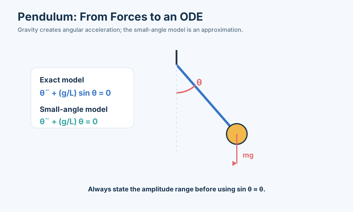
Forces: the pendulum
The exact restoring term is nonlinear. The familiar linear oscillator appears only after declaring the small-angle approximation.
For a mass on a rigid rod of length, torque balance gives
For small angles,, so
The approximation has a domain. Comparing the nonlinear and linear models across initial angles is a validation of the simplification.
Build the pendulum equation from motion
Stand beside the picture and decide where angle zero is: the mass hangs straight down. If we displace it to a positive angle, gravity pulls it back toward zero. The component of gravity tangent to the circular path has magnitudeand acts in the negative angular direction. Distance along the circle iswhenis in radians, so tangential acceleration is. Newton’s second law along the tangent gives. Divide byto obtain. That negative sign is physical: when the bob is to the positive side and briefly at rest, it accelerates back toward the center.
The pendulum’s state needs two entries, angleand angular velocity. Writeand. If the bob is released from rest at 10 degrees, the initial conditions areradians and. A release from 60 degrees with a push requires a different initial velocity; merely specifying the angle would not choose one trajectory. This is why the first-order state form helps a beginner see what initial information a second-order law needs.
Unit-check the coefficient.has metres per second squared,metres, sohas per-second-squared units. Radians are dimensionless for this check, hencehas angular acceleration units. Notice that masscanceled. In the ideal rigid-rod, point-mass, no-drag model, heavier and lighter bobs of the same length have the same period. If a real experiment shows a strong mass effect, investigate drag, bob geometry, or pivot friction instead of inserting mass into the ideal formula without a mechanism.
The exact restoring term is, not. Why do school formulas use? Near zero, the sine curve and the line through the origin agree closely. At 10 degrees,; the linearized restoring acceleration is about half a percent larger in magnitude. At 60 degrees, the ratio is about; replacing sine by angle overstates the restoring term by much more. The small-angle approximation is a controlled simplification when release angles are small, not a second law of physics. A nonlinear simulation can show that larger-amplitude oscillations take longer than the small-angle period, even in a frictionless ideal pendulum.
For the linearized equation, release from rest at anglegives. One full oscillation advances the cosine argument by, so. A one-metre pendulum withhas small-angle period about two seconds. A four-metre pendulum has period about four seconds, not eight, because period scales with the square root of length. Mass and small release angle do not appear in that approximation. Reading parameter dependence from the formula is more useful than memorizing its letters.
There is a powerful check for the ideal nonlinear equation. Kinetic energy isand gravitational potential relative to the hanging position is. Their sum should remain constant when there is no drag, motor input, or pivot loss. Numerically differentiate the sum along a simulated trajectory or compare its start, midpoint, and later values; a large drift indicates a numerical or coding problem. If we add damping proportional to angular velocity, energy should instead decline, so preserving energy would be the wrong validation criterion. The check follows the physical mechanism stated in the model.
What would we measure to decide whether the small-angle simplification is adequate? Release the same pendulum at several known angles, record crossing times and amplitude, and compare measured periods with both the small-angle prediction and the nonlinear numerical model. If amplitudes decay due to air drag, include that effect or focus on early swings. A modeler should not label every period mismatch “solver error”; some mismatch is expected because the linear approximation deliberately dropped higher-angle behavior. The pendulum gives us our first full derivation family: forces determine a rate of motion, initial angle and velocity select a path, and an energy or period check tests what we claimed.
Why a real swing gradually stops
The ideal calculation predicts a bob that swings forever because it has nowhere to lose mechanical energy. A real bob pushes air aside and rubs at its pivot. If observed peak angles shrink from swing to swing, the energy-conservation check is not “failing”; the model has omitted a loss mechanism. One common first extension treats the resisting torque as proportional to angular velocity:, with. The angular equation becomes. In the two-state form,and. The damping term always opposes current motion: whenit contributes negative angular acceleration, and whenit contributes positive angular acceleration. This sign behavior is more reliable than remembering a plus or minus from a textbook line.
The ideal energynow changes at rate. We can derive that by differentiating both energy terms, then substituting the damped equation. This gives a new numerical check: energy should decrease or stay momentarily flat when, never rise spontaneously in a closed damped model. If a computed trajectory gains energy on every swing without a motor or external forcing, the code is wrong or its time step is too coarse. The damped model also shows that validation criteria must match the assumptions. Applying the frictionless “energy constant” test to a frictional model would reject correct behavior.
At small angles, the damped law is approximately linear:, withand. For light damping, peak amplitudes decay roughly likewhile oscillating. We might estimatefrom successive measured peaks andfrom direct measurement, then compare predicted times of zero crossings. But “proportional to angular velocity” is an assumption: dry pivot friction may have nearly fixed magnitude and change sign with motion, while drag at higher speeds may be closer to quadratic. If peaks shrink in a pattern the linear-damping law cannot explain, fitting a different value ofwill not repair its structure. The appropriate extension depends on what the data show.
There is a small but useful lesson about names here. Calling the undamped periodan observed period for a large, damped release mixes two approximations. We can use it as a first estimate, then say which assumptions its error tests: small angle, light damping, rigid length, point mass, and fixed gravitational acceleration. When a 60-degree release disagrees, the sine approximation is an obvious suspect; when amplitude declines strongly, dissipation is another. A modeling answer is strongest when it can name why it might be wrong before seeing the final graph.
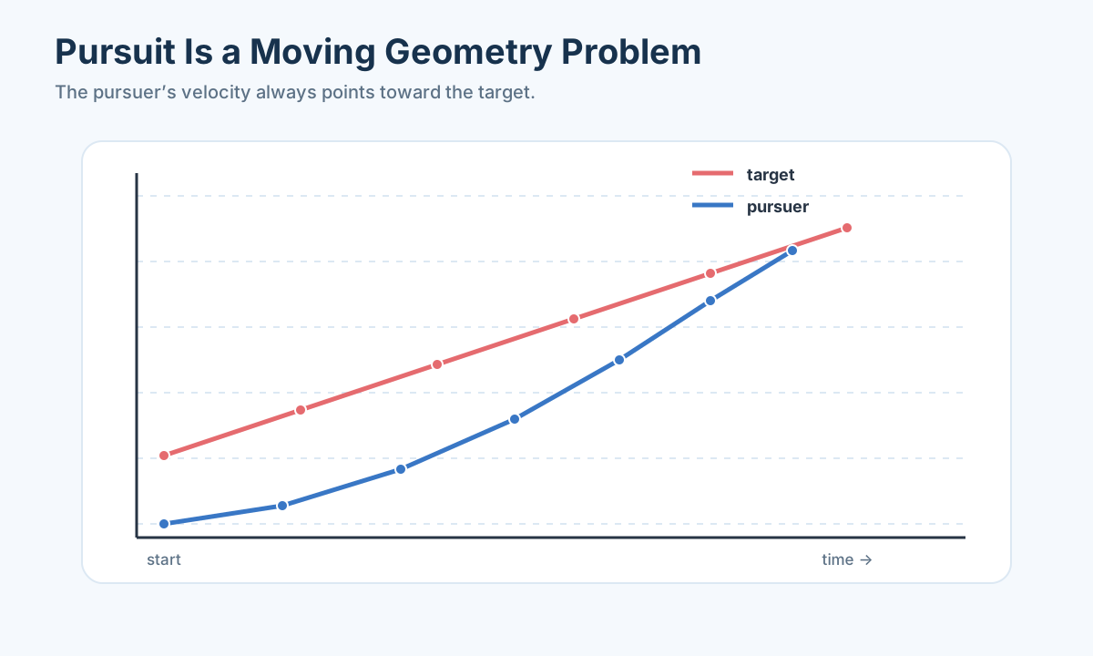
Geometry: pursuit curves
The target and pursuer must share one coordinate frame; the direction of the pursuer’s velocity changes continuously.
If a pursuer atalways moves toward a target atwith speed,
The target has its own motion law. Capture time is an event defined by, not just the end of an arbitrary simulation interval. Check whether speeds and geometry make interception possible.
Place both vessels on one nautical chart
The slide says a patrol craft and a submarine detect each other at the same time, initially 60 nautical miles apart. The submarine can travel at up to 30 knots and the patrol craft at up to 60 knots. A knot is a nautical mile per hour, so the units already tell us how to translate speed into position changes. Put the patrol atnautical miles and the submarine at. This coordinate choice is not a claim about north or east; it puts their initial separation on the horizontal axis to simplify reasoning. Both positions must be expressed in the same chart frame.
Before choosing a chase law, ask what the submarine does. If it travels straight away along the horizontal axis at its maximum 30 knots and the patrol follows directly along that axis at 60 knots, their separation isnautical miles. They meet after two hours under instantaneous acceleration and no turn limits. This is a benchmark, not the answer to every possible escape heading. Faster pursuer speed alone does not determine a unique intercept time because direction, detection delay, and control decisions matter.
Now suppose the submarine instead travels straight upward at 30 knots, so. If the patrol knows that heading and may turn instantly at constant 60 knots, a lead-intercept tactic aims at the future meeting point. The patrol can reachin timeif the distance from its start to that point equals:. Square both sides:, henceandhours. The meeting point isnautical miles. This hand calculation gives a comparison policy under a known fixed target heading. It is not the same as aiming at the submarine’s current position every moment.
Pure pursuit uses a different rule: at each instant the patrol’s velocity points toward the target’s current location. Write the displacement. Dividingbymakes a direction vector of length one; multiplying by 60 knots gives the patrol’s velocity. If the submarine moves sideways, the line of sight rotates, so the patrol traces a curve rather than the direct lead path. We cannot get its precise capture time from the 60- and 30-knot numbers alone; we must specify the target path, initial states, and control law and then solve or integrate the coupled equations.
The pure-pursuit equation also hides a singularity at exact capture: if, the denominatoris zero and the direction to the target is undefined. A numerical simulation should stop when separation falls below a declared capture radius, such as a physically justified sensor or interception distance, rather than taking one more derivative at zero. If an output grid records positions every minute, the true crossing can happen between grid points. Event detection is more accurate than calling the first sampled distance below threshold “the exact intercept time.”
We should challenge the model at the same time we use it. The submarine may dive below the patrol’s observation horizon; the patrol may not know its later heading; both vessels have turn-rate and acceleration limits; and currents can move them. A rule that points at a perfectly observed instantaneous target is a useful baseline but cannot be treated as a guaranteed real pursuit strategy. One extension could include patrol headingas a state and limit, so the craft cannot rotate instantly. Another could model delayed or noisy target position and optimize a lead point based on a filtered estimate. Each extension changes the question and needs data.
The chart example is a geometry-derived ODE, not a conservation ODE. Position changes according to a velocity direction set by relative geometry. In the water vessel next, stored volume changes according to an outflow set by gravity and geometry. The two mechanisms differ, but their modeling discipline is identical: name the state, put variables in one frame and unit system, define initial conditions, and stop at a physical event rather than at an arbitrary plotting time.
Turn the chase law into a checkable simulation
One reason I used both direct-away and sideways target headings is that they provide hand-calculated reference cases before a curved-pursuit simulation. A practical first experiment can take the submarine to move straight upward:nautical miles. The patrol starts atwith speed 60 knots and turns instantly toward. Carry the patrol’s two coordinates as statesand. At each evaluation time, computeand, then. The derivatives areand. Both derivatives have nautical miles per hour, and their squared sum has square root exactly 60 knots while. A calculation that gives patrol speed 90 knots after turning has normalized the direction incorrectly.
The first derivative evaluation can be done without software. At, displacement isand distance is 60 nautical miles, so the patrol initially moves atknots. After a short interval, the submarine has risen on the chart and the direction to it acquires a positive vertical component. The patrol’s path must therefore bend upward. If a plotted pure-pursuit trajectory begins by moving down or immediately toward the future intercept point, check coordinate signs or whether the code implemented a lead law instead of pure pursuit. We can test the direction law by recording patrol speed at each sampled state and the separation, not just by admiring the final meeting point.
For a capture event, defineand stop when it crosses zero downward. The thresholdshould be specified in nautical miles—perhaps a simplified radius for a rescue, sensor contact, or docking event. Its value affects reported time, especially if vessels cannot occupy precisely the same location. If you setin an equation containing, the event can be numerically fragile at the singular endpoint. Try two small meaningful thresholds and report the difference, then describe why this is a modeling convention rather than a solver defect. An event time is far more honest than “they meet on frame 45 of an animation.”
The lead-intercept calculation gavehours as a comparison. Since a lead strategy uses perfect advance knowledge of a straight target heading and flies a direct route to the eventual point, pure pursuit should not beat it under the same ideal speed limit. If your pure-pursuit code announces capture sooner than that benchmark, investigate whether it traveled faster than 60 knots, used future target location unintentionally, or mixed hours and seconds. Do not interpret the benchmark as a universal optimum under every real control limit: if patrol turning takes time, a direct route selected at the start may be infeasible; if target heading changes, the forecast may be wrong. The value is a unit test for the toy comparison, not a naval tactics claim.
We can now make the assumption of instantaneous turning explicit. Let the patrol’s heading bemeasured from the horizontal chart axis. Its position law becomesknots. If heading can change at mostradians per hour, we need a heading-rate controlwithand. The state has grown from position alone to position plus heading because two patrols at the same location but facing different directions cannot have the same short-term future. The “point directly at the target” policy can be approximated by turning toward the bearingas fast as allowed, but the exact control law must say how it handles bearing wraparound and what happens at capture. We have not chosen an optimal policy merely by writing down a turning bound; we have made one missing physical restriction visible.
Detection delay matters in a similarly concrete way. If the patrol hears the submarine at time zero but requires ten minutes to estimate its position, the submarine at 30 knots can travel five nautical miles before the patrol commits to a heading. If the patrol instead knows only an uncertain bearing, its predicted position is a region, not a point. A useful report might compare capture time over several target headings and delays, or show a probability of interception under a stated uncertainty model. But it should never turn the slide’s two speeds and 60-mile distance into one “correct” capture time without those choices. This is an example of a differential equation helping us expose the decisions that the original story left unspecified.
The pursuit curve described changing geometry. A draining vessel asks a different question: what quantity is stored, and where does it go? Keeping that distinction in mind will make the water-height equation feel like a balance rather than a formula to memorize.
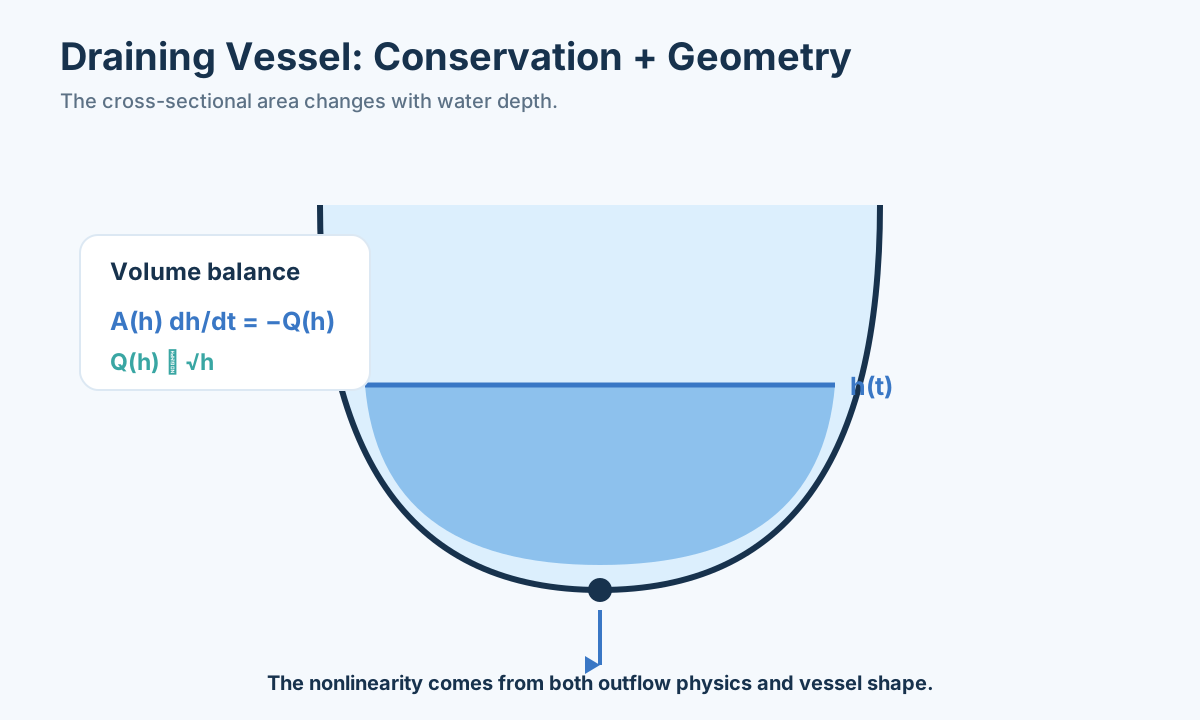
Conservation: a draining vessel
Conservation supplies the balance equation, while vessel geometry and outlet physics supply its nonlinear terms.
Letbe water depth. Conservation gives
whereis the vessel’s cross-sectional area andis outlet area. Geometry supplies; Torricelli’s law supplies outflow. A hemispherical vessel therefore differs from a cylinder even with the same initial volume.
Why the round bowl changes the answer
Picture a bowl whose inside is half a sphere, with its lowest point at the outlet. Let its radius be, and measure depthupward from that lowest point. At the bottom, a tiny rise in level adds little water because the horizontal slice is small. Near the top, the same rise adds much more because the slice is wide. This is the feature the cylindrical shortcut misses. We can get the slice area without memorizing a special formula. In a cross-section of the sphere, a pointabove the bottom is at vertical coordinaterelative to the sphere’s center. If the slice radius is, then. Rearranging gives, and multiplying bygives. Check the endpoints:at the point-shaped bottom andat the circular rim. Those two checks are a quick defense against copying the wrong geometric expression.
The volume below depthfollows by adding slices:. At the full-rim depth, this becomes, the familiar half-sphere volume. There are two equivalent ways to express accumulation. We can write, or use the chain rule. The second form tells us directly why the area belongs on the left of the level-change equation. A larger horizontal slice requires more water loss to lower the surface by the same amount.
Now specify the outlet. The ideal velocity from a headis approximately; an actual jet has a discharge coefficientthat absorbs contraction and other losses, sofor outlet area. Consequently. The equation combines three ideas, each with a job: geometry converts level into volume, conservation sets accumulation equal to negative outflow, and the outlet law relates outflow to head. If a pump supplies, the right side becomes. We do not need to change the geometric part merely because a pump was added.
Estimate the emptying time, not just the initial rate
Suppose the bowl starts full at. Rearrange the differential equation so a small fallcorresponds to a small elapsed time:. Summing those intervals from top to bottom gives
You can check the algebra by integrating the two powers separately:contributes, whilecontributes; their difference is. The result scales as, not as. Doubling outlet area halves this idealized emptying time, while doubling bowl radius multiplies it by. Size changes both the quantity stored and the gravitational head, so a linear radius rule would be suspicious.
For a hand-scale illustration, takemetre, a one-square-centimetre outletsquare metres,, andmetres per second squared. The formula predicts aboutseconds, or roughly 32.5 minutes. This is an invented illustrative bowl, not a measured classroom experiment. Treat the number as a way to check a simulation and expose the role ofand. If the hole becomes submerged by downstream water, the pressure difference changes; if the coefficient changes with flow regime, one constantwill not fit the entire trace. Measure several levels and times, then ask which assumption is failing before tuning a solver.
There is a numerical subtlety near empty. Bothandapproach zero as, but not at the same rate. The level derivative can become very steep near the bottom because the remaining horizontal slice is extremely small. An integrator may take tiny steps or report a value slightly below zero. Stop at an eventrepresenting the outlet geometry or a physically meaningful depletion threshold; compare the computed time with the integral. Do not ask a numerical routine to give a physically precise final microsecond from an ideal equation whose coefficient and outlet detail are approximate. The derivation is valuable precisely because it separates mathematical behavior from actual measurement accuracy.
Decide when to refill rather than waiting for empty
In practice someone may care less about the theoretical emptying time than about the moment a pump must begin to refill the bowl. Suppose the operating rule is “turn on the pump when depth first reaches.” The bowl’s changing area means halfway down in height is not halfway through its stored volume. At, the volume formula gives. The full bowl held, so onlyof its starting volume remains. A manager who calls “half-height” a “half-full” trigger would wait too long if the real constraint is stored volume. We need to state whether the sensor responds to height and whether the decision is based on volume, available pressure head, or a safety margin.
We can also compute the time to a chosen depthby integrating the sameexpression only fromdown to. Define. Then. No new differential equation is needed; we only change the stopping event. A numerical implementation should agree with this expression for the ideal assumptions. If a refill pump starts at the threshold, the later water depth obeyswhile the pump runs. The outflow law may stay the same, but the state now experiences a piecewise input.
Suppose the pump delivers a constant positive volume rate. At a given depth, compare its inflow with outlet outflow. If, depth rises; if it is smaller, depth continues falling despite the pump being on. An equilibrium depth would satisfy, givingif that value lies within the bowl. Because outflow increases with head, a fixed pump could eventually balance the outlet. The formula is a warning, not a substitute for operating data: pump rate can depend on pressure, and a pump may switch off at another threshold. A complete controller must specify both on and off rules, or the model will not know when the input changes.
If the pump turns on atand off at, the two thresholds create hysteresis. That word sounds technical, but its purpose is simple: one on/off threshold can make a noisy sensor flip the pump rapidly near that level; separating start and stop levels creates room between decisions. The system’s state must now include whether the pump is currently on, because identical depth can be encountered once during drainage with the pump off and once during refill with it on. Height alone no longer determines the next rate. We have discovered state memory through a real operational rule, exactly the issue we raised at the start of the lesson.
To test this control model, watch one real cycle: depth, pump state, and time stamps. Does the pump actually begin near the declared threshold? Does height reverse direction after it starts? Does the measured rise match the estimated inflow-minus-outflow rate? A model that gets emptying time right but gets pump cycles wrong may still be useless for the decision. We should validate the event and the controlled regime, not only the free-drain equation. The same distinction reappears in inventory replenishment, traffic signals, battery charging, and disease interventions: a continuous state changes under rules, and switching events alter its derivative.
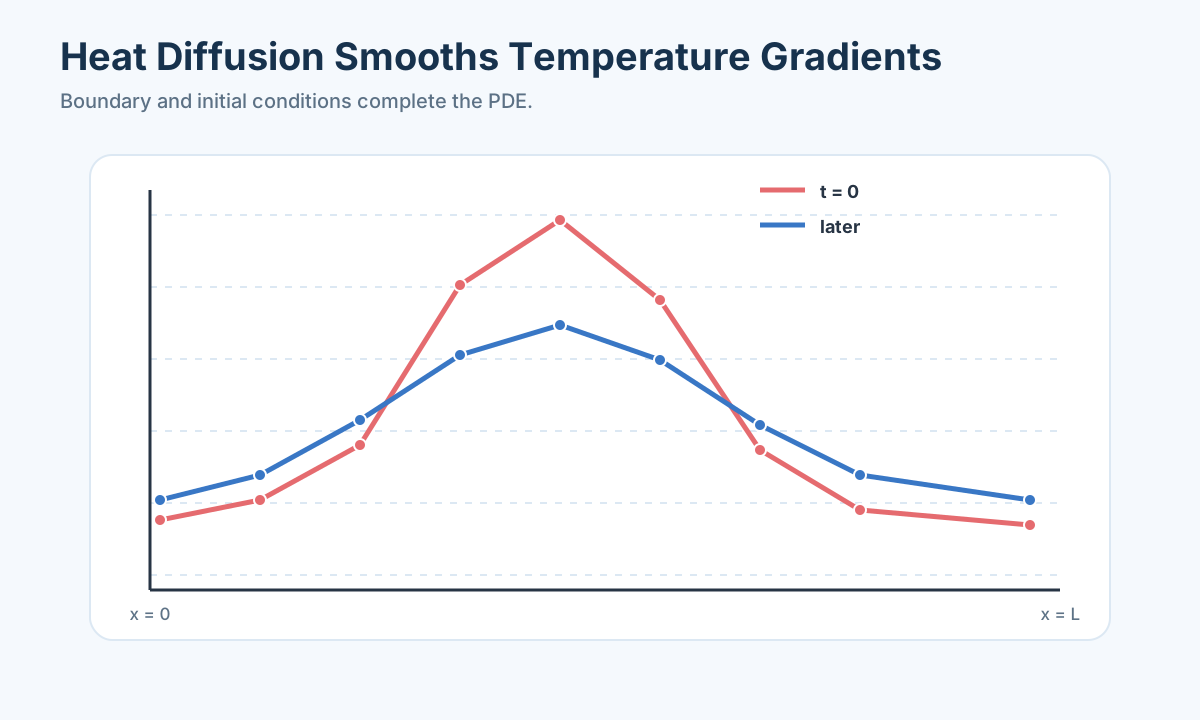
Distributed systems: heat conduction
Diffusion progressively smooths sharp temperature gradients. Boundary and initial conditions determine which solution is relevant.
A long rod with spatially varying temperature requires a partial differential equation,
For steady state,, reducing the model to an ODE in. Boundary conditions such as fixed endpoint temperatures complete the problem. This example shows why the independent variable need not be time.
Follow one small piece of metal
Why should temperature have a second spatial derivative? Imagine cutting a very short piece of rod betweenand. Heat conducted into its left face need not equal heat conducted out of its right face. Their difference warms or cools that piece. Fourier’s law says conductive heat rate across a face is, whereis conductivity andthe rod’s cross-sectional area. If temperature decreases toward the right,is negative and the heat rate is positive toward the right, as expected. Subtract outgoing from incoming conduction and divide by length: the result is. A curved temperature profile means the two end fluxes are different. A straight profile means those fluxes are equal.
The piece also loses heat from its exposed side to surrounding air. If the perimeter of the cross-section isand the air is at, the exposed area of the small piece is approximately. A simple convective-loss law assigns it rate, witha heat-transfer coefficient. The heat stored per degree of temperature change is, with densityand specific heat. Put these parts into “storage rate = conducted in minus conducted out minus side loss,” divide by, and obtain. The compact equation above uses the same balance after division by. It is a partial differential equation when bothandmatter.
Suppose we wait until every location stops changing in time while two heaters maintain endpoint temperatures. Thenand. This steady-state equation is an ordinary differential equation in position, but it still needs two endpoint conditions:and. An initial rod temperature is not needed to specify the final steady profile; it is needed if we ask how long the rod takes to reach that profile. Mixing those two questions gives apparently plausible but uninterpretable calculations.
Solve a two-ended rod without hiding the assumptions
Setso thatmeasures temperature above ambient. Let, whose units are inverse length squared. The steady equation becomes. Hereis a spatial decay parameter, not the bob’s mass from the pendulum. For fixed endpoint temperaturesand, one convenient form of the solution is
Check it before trusting it: at, the first fraction is one and the second zero; at, the first is zero and the second one. Each endpoint therefore receives exactly its specified temperature. Inside the rod, both endpoint influences decay because heat escapes to the surrounding air. If, thenand; the solution tends to the straight-line interpolation between endpoint temperatures. That limiting case is an excellent unit test for a coded formula. If a purported no-loss solution still curves toward ambient, its equations or implementation are wrong.
Letmetre,per metre,,, andas illustrative values. Halfway along the rod, both hyperbolic-sine weights equal. The midpoint’s excess temperature is therefore, or total temperature about. If the sides did not lose heat, straight interpolation would giveat that same point. The difference is not a mysterious curve-fitting choice; it is the energy carried away by the air along the rod. Before using the numerical value in a real device, one would measure,, geometry, and the actual ambient temperature.
How would we decide whether this model is sufficient? Put temperature sensors at several interior locations. A constant ambient-air temperature and constant convection coefficient are simplifications; a fan, insulated patch, or varied cross-section could cause deviations. If the measured profile disagrees mostly near one boundary, check whether the endpoint temperature is truly fixed or whether the heater itself has contact resistance. If the profile changes over time, the steady equation is answering the wrong question and we must restore the storage term. A more elaborate model is justified when it explains these residual patterns, not merely because it produces a prettier temperature plot.
If the heater has just been switched on
Suppose both rod ends are suddenly held at their new temperatures at noon. A steady profile predicts where the rod eventually settles, but it does not predict the first minute. To ask about that minute, specify the rod’s initial profile, perhaps uniform at, and keepin the balance. Temperature now depends on both position and time. The endpoint conditions say what the heaters enforce atandfor later times; the initial profile says what energy was stored before heating. If a modeler supplies only the two endpoint temperatures to a transient solver, infinitely many initial interiors are still possible. Different initial interiors can share the same final steady solution but warm up along different paths.
For a quick sanity check, imagine the left end is hot and the interior initially cold. Heat should begin to spread inward from the left. If the model predicts the interior becomes hotter than both heaters immediately, examine sign conventions, units, boundary treatment, and whether a heat source was added without explanation. With no side loss and fixed endpoints, heat diffusion smooths differences; it does not create heat from nowhere. With side loss, the room also drains energy. That verbal picture is what the minus sign onencodes when the rod is hotter than ambient. If the rod is colder than ambient, the same term becomes positive: the room warms the rod. A sign that works only for the hot case is not a general physical law.
We can turn the spatial equation into many coupled ODEs by dividing the rod into cells. Let cell-center temperatures beseparated by distance. Approximate the curvature at an interior cell by. Its rate equation has conduction from adjacent cells and side loss toward ambient. For a cold cell between hotter neighbors, that numerator is positive, so conduction warms it. For a hot cell between cooler neighbors, it is negative, so conduction cools it. We have reduced a PDE to an ODE system, but the approximation depends on grid size. Halvingshould not drastically change a decision-relevant temperature crossing time if the grid is already fine enough. If it does, refine further or inspect the model’s boundary treatment.
Numerical stability deserves attention here. In a simple explicit time-stepping method without side loss, a one-dimensional heat grid has a familiar scale: its step must be small relative todivided by thermal diffusivity. A finer spatial grid can force much smaller explicit time steps. This is one reason discretized diffusion can appear stiff. An adaptive implicit ODE solver can help, but we should still compare against the steady analytic profile at late times, test whether total energy behaves consistently with boundary input and side loss, and check grid refinement. A solver’s success flag does not validate the physical boundary conditions we chose.
The same workflow applies to other distributed systems. A chemical diffusing through tissue, traffic density changing along a road, or a contaminant moving through soil has both location and time. What counts as the state is a field, not one scalar. Boundary conditions specify what can enter or leave at the edges; initial conditions specify what was there at the beginning. The rod is an accessible physical example because we can touch the two ends, point to the surrounding air, and see why each term should be present. In a new PDE, I would look for an equally concrete local balance before trusting a memorized equation.
The four slide examples now differ in what supplies the rate. For the pendulum a force changes motion; for pursuit relative position sets velocity direction; for the bowl a volume balance changes water level; for the rod a local heat balance changes temperature. This is the organizing principle I want you to carry into a new modeling problem. Ask what changes, what mechanism pushes it, what condition chooses the particular path or profile, and what cheap physical check would catch a sign error.
We have met mechanics, pursuit, flow, and heat. Their symbols and units differ, but each can be rescaled so its dominant time and length scales become visible. This is why we step back from four examples and study dimensionless groups.
Nondimensionalize
Choose characteristic scalesandand set,. Dimensionless groups reveal which mechanisms dominate and reduce the number of independent parameters. They also improve numerical conditioning.
Rescale the tank so the shape of its answer is visible
The symbol change can look like needless algebra, so let us perform it on the cylinder that we already solved. Its level satisfies, withand initial depth. Define a fraction of starting depth. This is a quantity between one at the start and zero when empty, independent of whether the tank started at one metre or ten. Define a fraction of the ideal emptying time, where. Substituteandinto the rate law. The factors cancel and leavewith.
That equation has the simple answerfor. In these coordinates, every cylinder with the same flow law and no inflow follows the same normalized level curve. A tank twice as wide or with a smaller hole changes the clock scale, but not the shape after we divide time by its own predicted emptying time. At one quarter of that time,, so more than half the original height remains. At halfway, only one quarter remains. This is not because the second half of the tank is physically smaller; the level-versus-time curve reflects slowing outlet velocity. A normalized plot is often a better comparison of several experiments than a plot with raw time axes that hide the common mechanism.
The equation also tells us which changes cannot be absorbed into one time scale. A bowl has depth-dependent, so its normalized curve is different. A pump adds an inflow term, and a submerged outlet changes the head relationship. If measured normalized cylinder traces fail to lie near, a parameter-rescaling excuse is insufficient; there is missing physics or a measurement problem. This is why nondimensionalization is a scientific comparison tool, not only a trick to give a solver numbers near one.
Compare a swinging bob and a warm rod in the same spirit
For the pendulum, use dimensionless time. The exact ideal equation becomes. Gravity and length have moved into the conversion between physical seconds and the dimensionless clock. If two ideal pendulums are released from the same angle with the same dimensionless initial angular velocity, their angle curves coincide after rescaling time. If release angles differ, nonlinear amplitude effects remain; no time conversion makes a 60-degree swing identical to a 5-degree one. The approximationis therefore a statement about a dimensionless state, not about making seconds small.
For the steady rod, use position fractionand temperature excess. Since, its equation becomes. The productis dimensionless. It compares rod length with the characteristic distanceover which temperature influence decays under side losses. Ifis much smaller than one, the profile is nearly straight between endpoints; if it is large, ambient loss bends the interior profile strongly. A long thin rod in moving air may have a largeeven with the same endpoint temperatures as a short insulated rod. We have condensed several physical inputs—conductivity, exposed perimeter, cross-sectional area, convection, and length—into one group that explains the profile’s shape.
Unit checks are embedded in these groups. The tank clock has seconds,is unitless, andis unitless becausehas inverse metres. If a proposed dimensionless group still has kilograms or seconds left after cancellation, its construction is wrong. In practice I would first put every quantity in a small unit table, then substitute scales. The algebra is much easier when the measurement story is clear: “level relative to starting level,” “elapsed time relative to time to empty,” and “position relative to rod length” are ideas you can explain without symbols.
Numerical solution and events
Numerical integration should report method, tolerances, time span, evaluation points, and event conditions. SciPy’s solve_ivp solves first-order initial-value systems and supports event detection and multiple algorithms (official documentation ).
Validate by reducing step size or tolerances, checking conserved quantities, comparing with an analytic special case, and testing limiting behavior. A visually smooth curve can still be numerically wrong.
First compute one step in ordinary language
Before passing a derivative function to software, take a tiny forward step by hand. For the cylinder atmetre, we foundmetres per second. A crude one-second forward-Euler estimate ismetre. At that new height the derivative is slightly smaller in magnitude because. If an implementation reports an increase tometres, the sign is reversed. If it reportsmetre after one second, the unit conversion, outlet area, or time scale is suspect. One hand step is not the final simulation, but it isolates the meaning of the derivative function better than staring at a polished curve.
Euler’s method repeatedly applies. It is easy to explain and is useful for checks, but a largecan miss curvature, overshoot a boundary, or make a positive state negative. Modern adaptive solvers estimate local error and adjust internal steps. A request for output at every minute does not necessarily force an adaptive solver to take exactly one-minute internal steps; it specifies the times at which we want reported values. Distinguish the numerical work from the plotting grid. If we care about the instant a tank crosses a pump threshold, ask for an event root, not only a sparse sequence of reported water levels.
Imagine a pump that starts whenfalls belowmetre in the cylindrical example. The exact normalized curve gives. Withmetre, setto obtain, so the ideal crossing occurs at half the emptying time, about 376.5 seconds. A plot sampled at 300 and 420 seconds can show the crossing is somewhere between, but it cannot by itself tell you the switch time. A root-finding event evaluates the continuous numerical solution between its internal steps. Use a downward-crossing direction if the pump should trigger on falling level; otherwise an upward oscillation could accidentally trigger the same event. Once the pump turns on, its inflow changes the differential equation, so the simulation becomes a sequence of regimes rather than one unchanged curve.
Select a solver from behavior, not prestige
For many smooth non-stiff models, an adaptive explicit Runge–Kutta method such as the default RK45 in SciPy is a sensible start. The routine solve_ivp expects a function that returns derivatives at the requested time and state. A second-order pendulum must first be converted to the two-state system; a pursuit model might carry four position coordinates; the hemisphere has one height state until the outlet law changes. Choose a time span that includes the physical event and an initial state that carries the right units. Look at the solver’s success flag and message, not merely at whether arrays of numbers exist (SciPy’s solve_ivp reference).
Tolerance settings are not magic accuracy certificates. Relative tolerance weighs error in proportion to state magnitude; absolute tolerance matters near zero. If one state is water depth in metres and another is a pollutant mass in micrograms, default tolerances can treat them unevenly. Scale states or give appropriate componentwise tolerances when the API permits. Re-run with stricter settings and compare the decision—capture time, pump-trigger time, safe-temperature crossing—not just whether two lines appear to overlap. A one-second shift may be invisible on a 24-hour plot but important for a control action.
Some equations are stiff: one component changes so fast that an explicit method must take tiny steps even though the slower behavior is what we care about. An implicit method such as Radau or BDF can be more efficient in those cases. A rod-heating model with very fine spatial discretization can produce fast and slow modes; a chemical model may combine rapid reactions with slow transport. We should diagnose this from physical time scales and solver behavior. Do not select BDF because the equation looks difficult, and do not assume a smooth curve means no stiffness or no modeling error.
For the four slide examples, there are cheap independent comparisons. The ideal pendulum should conserve energy; a small-angle simulation should agree with its cosine formula at small releases. The direct-away chase should match the two-hour closure calculation before we attempt a curved target path. The cylinder should match its analytic emptying time; the hemisphere should match its separate integral. The steady rod should approach a straight line as convection tends to zero. If a codebase passes all of these, it has not proved that real-world assumptions are correct, but it has eliminated many algebraic, sign, boundary, and numerical mistakes. Physical validation then requires observed data and an explicit statement of the omitted mechanisms.
A complete first numerical example uses the logistic model:
1
2
3
4
5
6
7
8
9
10
11
12
13
14
import numpy as np from scipy.integrate import solve_ivp
t_eval = np.linspace(0, 30, 301) sol = solve_ivp(logistic, (0, 30), [N0], t_eval=t_eval, rtol=1e-8, atol=1e-10) assert sol.success N = sol.y[0] assert np.all(N >= 0) and np.all(N <= K * 1.001)
Now repeat with tighter tolerances, compare the trajectories, and verify thatinitially grows almost exponentially and approaches. Those checks are part of the solution, not optional cleanup.
Derive and check an ODE
Suppose a room contains a pollutant with concentration, volume, clean-air inflow, and internal generation rate. Perfect mixing gives the balance
Every term has units pollutant mass/time. The left side is accumulation,is generation, andis removal. This “accumulation = inflow − outflow + generation” pattern is reusable in tanks, heat, finance, populations, and inventories.
Solve the simplest case by hand
For constantand,
The equilibrium isand the time constant is. After one, the difference from equilibrium is multiplied by. These interpretations are more valuable than the algebra alone. They tell us that doubling ventilation halves equilibrium concentration and response time.
Read the solution as a room, not as an exponential
Let us make the symbols tangible. Imagine a perfectly mixed workshop with air volumecubic metres. A process releases a harmless-to-illustrate tracer at constant ratemilligrams per hour, and clean air is exchanged at ratecubic metres per hour. Let the initial concentration bemilligram per cubic metre. The generation termis milligrams per hour. The removal termis, also milligrams per hour. Storageis milligrams, sois milligrams per hour. This unit balance is more informative than simply saying the equation has the right shape.
The new steady concentration ismilligram per cubic metre. Initially the workshop containsmilligrams of tracer. Production adds 10 milligrams per hour while ventilation removesmilligrams per hour, so concentration should initially fall. The differential equation agrees:milligram per cubic metre per hour at time zero. A crude one-hour Euler step would givemilligram per cubic metre. The exact expression gives, so the hand step is close but not identical. If a program predicts a rise, ask whether clean-air inflow was accidentally modeled as carrying tracer or whether generation and removal signs were swapped.
The time constanthours says how quickly the difference from equilibrium decays, not how long until concentration becomes exactly equal to equilibrium. After five hours,milligram per cubic metre. After ten hours,. Mathematical exponential decay approaches its equilibrium asymptotically; a practical decision needs a threshold, such as “below 0.7 milligram per cubic metre,” with a stated reason for that threshold. Solvinggivesandhours. That is a physical event time. Sampling a graph hourly would only show that crossing somewhere between hours four and five.
What if we double ventilation tocubic metres per hour while leaving generation constant? The equilibrium falls tomilligram per cubic metre and the time constant becomes 2.5 hours. Starting from the same, after 2.5 hours the new solution ismilligram per cubic metre. Two effects happen together: the destination is lower, and the move toward it is faster. Saying only “twice the airflow halves concentration” describes steady conditions but misses the transient. For a class project about when a room can be occupied, the transient threshold may be the actual decision, not a steady-state number.
Perfect mixing is a strong assumption. A person sitting by the source might breathe air very different from a sensor by the door. Ventilation flow is not necessarily a uniform replacement of every cubic metre; a short circuit between supply and exhaust can leave stagnant zones. Generation may pause during breaks and surge when equipment starts. An observed rapid spike followed by a slow tail would tell us to inspect source timing, zone exchange, or sensor lag. We can extend the equation, but the baseline first reveals which mechanism an extension must explain. We would not claim an actual health or regulatory limit from this toy tracer scenario; its numbers are invented to practice balance, units, time constants, and threshold reasoning.
What can the measurements actually identify?
Suppose we record only one concentration long after the workshop has settled. The observation approximately gives. It does not separately tell usand: a release of 10 milligrams per hour with 20 cubic metres per hour of clean air and a release of 20 milligrams per hour with 40 cubic metres per hour have the same ratio. The two rooms can nevertheless reach that equilibrium at different rates becausediffers. A measured transient, together with known volume and a sufficiently clear starting state, provides information about the time constant; combining transient and steady measurements may allow both parameters to be estimated. This is an identifiability issue, not a failure of the algebraic solution.
Think about sensor placement and sampling before fitting parameters. If the true time constant is five hours but we measure only at the start and after thirty hours, almost all samples tell us about equilibrium and almost none show the early change. If all measurements occur within the first few minutes, they mostly reveal the initial derivative and may not pin down the eventual level. Samples distributed around one or two time constants are more revealing. We also need to know whetherstayed constant and whether incoming air truly had negligible tracer. Otherwise the fittedcan become a convenient label for several missing processes rather than a measured ventilation rate.
To fit data, write the predicted concentration at each observation time from the model, subtract prediction from observation, and examine the residuals. If residuals drift upward during working hours and downward overnight, constantis not explaining the schedule. If the residuals are systematically larger near the source sensor than the far sensor, perfect mixing is questionable. If all residuals are small butandchange wildly when one data point is removed, the fit is not robust. Plotting only predicted and observed lines on the same axes can hide these patterns; a residual plot is part of understanding the mechanism.
There is a helpful distinction between uncertainty in parameters and uncertainty in structure. A 10% uncertain flow meter gives parameter uncertainty inwithin the one-zone model. A poorly mixed room means the one-zone equation may be wrong even ifwere known exactly. Tightening a numerical solver’s tolerance will shrink neither uncertainty. For a decision threshold, test plausible,, and initial concentrations and report how much crossing time changes. If the threshold time changes drastically, propose a better measurement or a conservative policy. If it barely changes, the simple model may be good enough for the decision despite imperfect parameter estimates.
Convert higher-order equations to first order
Numerical solvers expect. For, defineand:
Initial position and velocity are both required. Missing initial or boundary conditions are a modeling error, not a solver setting.
Learn solver behavior
Explicit Runge–Kutta methods work well for many smooth, non-stiff systems. Stiff systems contain very different time scales and may force explicit methods to take tiny steps; implicit methods such as BDF or Radau can be more efficient. Diagnose stiffness from mechanism and solver behavior rather than choosing an implicit solver automatically.
Absolute tolerance controls errors near zero; relative tolerance scales with solution magnitude. Re-run with tighter tolerances and compare decision-relevant outputs, not only curves. Use event functions for threshold crossing, impact, depletion, or extinction so that the solver locates the time rather than relying on a coarse output grid.
Estimate parameters responsibly
If concentration observations are, estimateby nonlinear least squares or likelihood. Plot residuals versus time and fitted value. Profile one parameter while refitting the other to reveal correlation. Short observations may identifybut notandseparately; this is practical identifiability.
Extend only when evidence demands it
Perfect mixing may fail in a large room. A two-zone model adds near-source and far-field concentrations with exchange. Time-varying occupancy changes. Sensor delay adds a measurement model. Compare each extension against the simple model on held-out data and retain it only if it improves explanation or decisions.
A two-zone room when the one-zone assumption is visibly wrong
Imagine the source sits in a small work area beside a larger room. A sensor near the source sees a high concentration while a sensor across the room sees a lower one, even after both have stabilized. One average concentration cannot simultaneously explain those two readings. Divide the air into a near zone of volumeand a far zone of volume, with concentrationsand. Suppose tracer enters the near zone at rate, ventilation removes tracer from each zone at ratesand, and an exchange flowmoves air between them. A simple balance isand. Every term remains mass per time. When, the exchange term removes tracer from the near zone and adds it to the far zone, preserving total tracer under exchange alone.
Add the two equations and the exchange contributions cancel:. That cancellation is an independent conservation check. If a coded two-zone model creates tracer mass when we set, it has broken exchange symmetry. We can also check a limiting case: as exchangebecomes very large compared with other flows, the two concentrations should become close and the system should resemble a well-mixed room. Ifis tiny, the source area can remain much higher than the rest. These limits are useful before fitting any exchange coefficient to data.
The extra zone does not automatically make predictions more trustworthy. We now need separate or at least inferable volumes, ventilation allocation, exchange flow, and sensor positions. One pair of late steady readings may not identify every parameter. Observe a startup or a controlled tracer release and record both sensors over time; their different rise and decay rates carry information aboutand. Keep the one-zone model as a comparison. If the two-zone model predicts a held-out day noticeably better and changes the occupancy decision, complexity earned its place. If it merely reduces training residuals because it has more adjustable parameters, it has not yet demonstrated a better physical explanation.
How a time-varying source changes the story
Suppose the process releases tracer only when a machine runs, from 9:00 to 12:00 and again from 14:00 to 17:00. We can represent that schedule by a piecewise, zero during the breaks and positive during operation. The concentration need not settle at one permanent equilibrium. During operation it moves toward the corresponding operating equilibrium; during a break it moves toward zero if ventilation continues. A snapshot at 13:00 cannot be interpreted withusing the 9:00 operating rate as though the machine had run continuously. The ODE records the history of recent input through its current state.
If the machine starts at a known time, the solution for each interval can be propagated from the concentration reached at the previous switch. The concentration at noon becomes the initial condition for the lunch break, and the break’s ending concentration becomes the initial condition for the afternoon period. We do not reset to the morningeach time unless the room was physically cleared. This is an everyday version of a piecewise dynamical model: the rate rule changes at scheduled events, but the stored amount carries over. It resembles the pump’s on/off cycle in the water bowl, though the mechanisms differ.
When an observed sensor responds ten minutes after a source change, the room may not be slowly mixing; the sensor itself may average readings or report with a delay. A measurement model can sayfor delay, or model a sensor’s own response rate. Distinguish the hidden physical concentration from what the instrument reports. Otherwise the fitting routine may lower estimated ventilation to imitate slow sensor response, leading to the wrong airflow decision. Collecting information about sensor technology can be more valuable than increasing model order.
The room example helps bridge this lesson to the next. One concentration state was enough for a fully mixed space; two interacting concentrations were needed when exchange and local exposure mattered. In population modeling we will also divide a whole into groups when movement between groups changes the decision. Before drawing arrows between compartments, ask what is conserved by transfers, what enters or leaves from outside, and what observations can distinguish the groups. That is the same balance discipline learned from water and tracer, applied to people or organisms rather than fluid.
Practice
Derive the pollutant balance, solve the constant-input case, and verify the numerical solver against the analytic expression. Fitandto synthetic noisy data, calculate equilibrium and time constant, and test a step change in generation. Finally, create one dataset too short to identify both parameters and explain the ambiguity.
The workshop gave you a way to challenge an ODE. Let us return to the four slide pictures and match each picture to its state, rate, initial condition, and easiest sanity check.
Transfer the method to a new question
Imagine a small greenhouse just before a cold night. The owner asks whether the heater must run continuously or whether stored warmth in the air and soil can carry the plants through until morning. It would be tempting to take one temperature reading, subtract a guessed number of degrees per hour, and extrapolate to sunrise. But the heat-loss rate is not usually constant: it depends on how much warmer the inside is than outside, and the heater may turn on and off. We have not seen this greenhouse in the slides. That makes it a useful test of whether we learned the method rather than four examples.
Start with a minimal state: indoor air temperature. If the soil or building fabric stores a great deal of heat and responds slowly, one air temperature may be insufficient; for the first pass, state clearly that we ignore that storage. Let the greenhouse’s effective heat capacity bejoules per degree Celsius, let heater power when on bewatts, let ambient temperature be, and let an effective loss coefficient bewatts per degree Celsius. The balance is. Storage is joules per second, heater input is joules per second, and loss is also joules per second. If the greenhouse is warmer than outside and the heater is off,; if inside and outside are at the same temperature and the heater is off, this simple loss term predicts no immediate change. Those signs and limiting cases catch mistakes before we fit anything.
With constant outside temperature and heater off, write excess temperature. Thenand. The time constant is. If it is two hours, the excess temperature after two hours is about 37% of its starting excess. For an illustrative indoor start ofand outdoor constant, the indoor prediction after two hours is. But a real plant-safety decision might be whether temperature falls belowbefore the heater can respond, not merely the value after two hours. Solve or detect that crossing explicitly, and say where thethreshold came from.
Now ask what information the owner actually has. A thermometer provides, and a forecast provides an uncertain. The effectiveandmight be estimated from one night of heater-off cooling, but they may vary with ventilation, wind, humidity, and soil water content. If the heater turns on at a threshold, heater state becomes part of the evolving system; at the same temperature, a heater-on greenhouse warms differently from a heater-off greenhouse. Compare predicted and measured temperatures over several hours and look for patterns in the residuals. If the greenhouse cools quickly at first and slowly later, a one-state exponential might fit. If it cools slowly at first but plunges when a vent opens, the input or loss mechanism changed. If the temperature rebounds at dawn while the heater stays off, changing outside temperature or solar input belongs in the balance.
The first model need not solve every physical effect to be useful. It should answer a stated decision under stated assumptions and tell us which observation would force a revision. We have carried the tank’s storage-and-outflow reasoning to heat, the room’s time constant to temperature, and the pump’s switching logic to a thermostat. That transfer is the point of learning differential equations for modeling. The derivative is not an ornament added to make the answer look sophisticated; it expresses a changing balance whose future depends on state, conditions, and inputs.
There is a useful hand comparison before choosing a thermostat setting. For the illustrative greenhouse, the threshold is, ambient is, and the initial excess is. At the threshold the excess is, or one fifth of its starting value. With time constant two hours,giveshours. If the heater needs half an hour to become effective, a rule that switches on atwould be late under these assumptions. The owner might instead choose a higher switch-on temperature or a forecast-based trigger. The calculation does not dictate the rule by itself; it translates delay and thermal inertia into a question that can be tested with actual greenhouse data.
A forecasted outside temperature is rarely constant. If it falls fromtoafter midnight, the previous exponential formula with fixedno longer describes the whole night. We can solve separate intervals, using the indoor temperature reached at midnight as the next initial condition, or integrate the equation with a varying. This is another opportunity to test understanding: we carry the greenhouse’s stored temperature forward; we do not reset it to its original 20 degrees when the weather changes. Whether the threshold is crossed may depend on the timing of the cold front as much as on its lowest temperature. That is why a dynamic model can answer a decision that a single average-night temperature cannot.
Before presenting such a forecast to the owner, I would show three traces on one graph: measured indoor temperature from a previous night, the simple heater-off prediction, and a colder-weather scenario. All temperature axes would be labelled in degrees Celsius and the horizontal axis in clock time, not an unexplained solver index. The comparison would make the model’s useful range and the switching decision legible even to a teammate who never saw the equations.
Each rate law needs a state, units, and an initial or boundary condition. The next lesson uses the same accounting idea for interacting populations and compartments, where flows between groups make the dynamics easier to understand than a bare differential equation.