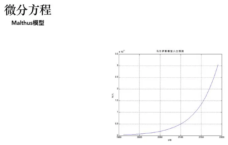
Yesterday’s differential-equation lesson described motion, flow, and heat. Now consider a population of people or products. If a new app has one hundred users today, can it keep doubling forever? Probably not: the pool of potential users is finite, and people influence one another. The first growth equation is useful precisely because we can see when it stops being believable.
We will begin with a simple population count, add a limiting capacity, and then split people into categories when one count is no longer enough. Susceptible and infected people, or unaware and active customers, belong in different “compartments” because their future changes differ. I will keep drawing arrows between stocks and reading each equation aloud as an inflow or outflow. When the fitted curve looks good, we will ask whether the observations can actually identify the rates behind it.
Many systems share a small number of dynamical motifs: unconstrained growth, saturation, transfer between compartments, and interaction between populations.
Malthus and logistic growth
If per-capita growth is constant,
This Malthus model is useful over short periods but grows without bound. Introducing a carrying capacitygives the logistic equation
Growth is nearly exponential when, fastest at, and approaches zero near. Do not fitfrom early exponential data and expect it to be identifiable.
Ask where the new people come from
Suppose a campus club has 100 members and is gaining roughly 10% of its membership per month. The naive but useful first thought is that every current member can recruit at a roughly constant average rate, so the club gainsmembers per month when its size is. The derivativesays just that. It is a rate statement, not a claim that members arrive in fractions. For large counts and a time scale of months, a continuous approximation can be serviceable even though recruitment happens one person at a time. Withandper month, the model gives. After one month that is about 111 members; after about 6.93 months it doubles to 200 because. A 10% continuous rate is not the same as multiplying by 1.10 once per month:. We can choose either convention, but we should not mix its parameter estimates.
Now ask the question the formula cannot answer: whom will the 10,000th member recruit on a campus with far fewer available students? If membership is limited by a pool, constant per-member recruitment cannot persist. A simple modification multipliesby the fraction of capacity still available,. Atthe rate is zero; whenis small compared withthe fraction is near one and we recover the early Malthus behavior. The logistic equation is not a magic law that all clubs obey; it is a hypothesis that the limiting mechanism acts roughly like the remaining fraction of one fixed pool. If the club loses members, admits graduates, or changes its recruitment campaign, those mechanisms need separate terms or time-varying parameters.
For an illustrative club capacity, starting atwithper month, the logistic solution is. Atthe denominator is ten and the answer is exactly 100. At the pointthe available fraction is one half, and the monthly derivative ismembers per month. Atthe derivative has fallen to. It is possible for the club to be gaining members more slowly at 900 than at 500 even though many more current members could recruit. The limiting pool is doing the work. For a student confused by an S-shaped curve, that calculation explains its bend.
Why is growth fastest at half capacity? Write the derivative as, a concave quadratic in. It is zero atand, and its vertex is at. At a tiny membership, there are many potential recruits but few recruiters; near capacity there are many recruiters but few potential recruits. Halfway balances those two factors. This interpretation is more memorable than taking another derivative mechanically. It also points to the logistic model’s assumptions: recruiters and available people interact in a fairly uniform way, the pool stays fixed, and the average rate does not depend on the club’s age or reputation except through.
Early observations may distinguish a rising curve from a flat one but tell us little about. If all measured values are between 100 and 150 whilemight be 500 or 5,000, the factoris close to one for both candidate capacities. Several values ofcan then fit nearly the same early data, particularly ifis adjusted at the same time. Claiming a precise eventual club size from only those early months would be unwarranted. Observe the slowing phase or collect independent evidence about the eligible pool before trusting. This lesson about what data can identify will return in epidemics, product diffusion, and compartment models.
A simple growth law is tempting because it fits a rising curve. Before using it for an innovation or product, ask what limits adoption and whether one person’s adoption changes another’s chance to adopt. That moves us from population count alone to a mechanism for spread.
The growth slide shows the tempting early exponential trend; the question for a forecast is where that trend must bend.
Adoption and product diffusion
A basic adoption model treats contact between adopters and non-adopters as the mechanism:
whereis market potential. External advertising can add a term proportional to the remaining market. The point is not that every product follows one S-curve, but that different mechanisms produce distinguishable rate equations.
One total population can hide crucial differences. In an epidemic, susceptible and infected people do not play the same role; for a product, aware and active users may not either. We now divide the total into stocks and draw the flows between them.
When adoption depends on both outsiders and friends
Imagine a new campus bike-share app. At first hardly anyone knows it exists, so a poster or announcement may create the first wave of users. Later students see friends using it and join through word of mouth. If we model only imitation asand start with exactly, adoption stays at zero forever: nobody can imitate a non-existent user. That is mathematically consistent but not a believable launch story when outside publicity exists. A small initial adopter group could fix the zero-start issue, but it would still hide the marketing mechanism. We can instead write a source term for external influence alongside imitation.
Letbe the fraction of potential users who have adopted, solies between zero and one. Bass diffusion uses $dF/dt=p+qFpqFF=0p1/2q/2F$ approaches one, both mechanisms slow because few non-adopters remain. If one wants the rate of new sign-ups, use, notitself; cumulative adoption and monthly sales are different outputs.
Try a hand calculation with illustrativestudents,per month,per month, and launch fraction. The initial rate isnew users per month in the continuous approximation. At, rate is $1{,}0000.02+0.30(0.5)=85F=0.91{,}000(0.02+0.27)(0.1)=29$ per month. The app can see sales accelerate and later decline while the cumulative user count continues to rise. That distinction matters for hiring support staff or buying additional bicycles. A cumulative S-curve alone hides the staffing peak.
The model is not a proof that advertising and word of mouth are the true causes of every rise and fall. A competitor could enter; a semester break changes student population; app quality can alter retention; new users may leave, so cumulative sign-ups are not the same as active users. If data include only monthly cumulative adoption, many combinations of,, andcan produce similar curves over a short early interval. Use incremental sign-ups, active-use counts, campaign dates, and independent market-size evidence to distinguish mechanisms. If growth jumps immediately after a marketing campaign even with few adopters,may matter; if new users track clusters of current users, imitation may matter. The model tells us what to look for, not what to believe without observation.
This product example connects directly to the previous club. Both have a finite remaining pool; the difference is whether adoption comes from current adopters alone or also from an external source. It also prepares the epidemic model. In an epidemic, people moving from susceptible to infectious are not “new people” added to the population. They transfer between states, and the interaction between susceptible and infectious people determines the flow. Drawing those distinctions before writing the equation prevents us from confusing the size of a group with the rate at which it changes.
Use the diffusion law to compare two launch choices
Suppose the bike-share manager can buy posters or fund a referral program. In the Bass law, posters mainly influence the external termwhile referrals mainly influence the imitation term, if those interpretations are supported by evidence. If we increasefrom 0.02 to 0.04 per month while adoption fraction is zero, initial sign-up rate in our 1,000-student illustration doubles from 20 to 40 per month. Increasingatdoes nothing at that exact starting instant because there are no adopters to imitate. Once half the market has joined, both interventions can matter, but they have different timing. This is not a proof that posters beat referrals; it is a question the model makes precise: when are existing adopters numerous enough for referral effects to propagate?
We should not decide by comparing only one instantaneous derivative. Poster spending has a cost, referrals may attract more retained users, and the market potentialmay grow or shrink. A fair comparison would specify a fixed budget, forecast sign-ups and active riders over a relevant term, and test plausible ranges forand. If the ranking changes under modest parameter changes, a small pilot campaign could teach us more than a grand forecast. If both strategies produce almost the same operational bicycle demand, the simpler or cheaper intervention may be enough. The rate equation helps frame an experiment and a decision, not merely draw a pretty S-curve.
Cumulative sign-ups are not active users
The bike-share app gives another reason to introduce compartments. Suppose 500 students have ever signed up, but only 200 currently use it. The diffusion model’scounted irreversible cumulative adoption. It cannot explain how people become inactive or return, becauseis not allowed to fall. Separate students into never-signed-up, active, and inactive-but-signed-up. A launch or imitation mechanism moves; churn moves; reactivation moves. The totalremains the potential student market if we ignore new enrollments and graduations. Each arrow should appear as a negative term in its origin stock and positive in its destination.
Let initial adoption flow be, churn rate, and reactivation rate. Then,, and. Sum the three equations to get zero. Cumulative sign-ups equal, whose derivative is; active users equal, whose derivative also depends on churn and reactivation. If a company buys bicycles based on cumulative sign-ups when most users have stopped riding, it may overestimate near-term demand. If it judges campaign success only by active users when a large new cohort is still onboarding, it may underestimate reach. The stock choice follows the decision.
There is a simple one-month arithmetic check. Start with,, andstudents in an illustrative 1,000-student market. Suppose 30 never-users join during the month, 20 active riders churn, and 10 inactive riders reactivate. Ignoring within-month rate variation, the month-end counts are,, and. Their sum remains 1,000. Cumulative sign-ups rise from 500 to 530, while active users rise by only 20. If a model reports sign-ups rising by 30 and total population rising by 30, it has added adopters rather than transferred them. The intermediate flows—30 joining, 20 leaving active, 10 returning—explain the difference between output metrics.
Estimating these flows requires more than a cumulative download counter. Account logs can track active status and reactivation, with a declared definition of “active” such as at least one ride in the last 30 days. Changing that definition will changewithout any underlying behavior changing. Student enrollment data reveal whetherchanges across semesters. If privacy rules prevent person-level tracking, aggregate transition data or repeated surveys might still constrain rates, but uncertainty should be reported. The model can guide production or staffing only if its compartments correspond to operationally measured states.
This is also a way to understand why copying a beautiful S-curve into every domain is risky. Product adoption, an epidemic, a radioactive sample, and predator-prey interaction can all produce nonlinear-looking time traces, but their arrows and conserved totals differ. Each equation is a compact claim about what changes and what cannot change. When a curve from a dataset surprises us, the first response should be to inspect those claims before searching for a more flexible mathematical shape.
Compartment models
Divide the system into well-mixed compartments and write one balance per compartment. For a substance moving between two compartments,
Arrows in the compartment diagram must correspond one-to-one with terms in the equations. This structure appears in pharmacokinetics, tracer studies, glucose–insulin models, material flows, and customer migration.
Draw arrows before guessing coefficients
Imagine that a harmless tracer is injected into the bloodstream. Letbe the amount in a central compartment andthe amount in a tissue compartment, both measured in milligrams. The inputis milligrams per hour. Tracer leaves the central compartment for tissue at rate, returns at rate, and is removed from the body at rate, where eachhas units inverse hours. This story gives the two equations above term by term. Thearrow appears with a minus sign in the central equation and a plus sign in the tissue equation. The return arrow appears with the opposite pair. Elimination appears only as a minus in the central compartment because it leaves the modeled system.
Add the two equations. Internal transfers cancel and leave. That is the whole-body mass balance. If we set input and elimination to zero, total tracer should remain constant even while it moves between compartments. A graph withfalling andrising might look plausible, but if their sum increases, the model has duplicated an arrow. This cancellation is a better test than checking whether each curve looks smooth. The same arithmetic applies to money transferred between accounts, students moving between course levels, and customers migrating from trial to paid status. Transfers do not create the thing being counted.
Consider a tiny hand step. Initiallymilligrams and. Letper hour,per hour,per hour, and input zero. At the initial instant, central-to-tissue transfer is 20 milligrams per hour, return is zero, and elimination is 5 milligrams per hour. Thusandmilligrams per hour, and whole-body amount declines at 5 milligrams per hour. A crude one-tenth-hour step givesand, total 99.5. That intermediate transfer number of 20 is the check: if code reports 2 or 200, inspect whetheror the time unit was misread. The step is an approximation, but the stock-flow identity is exact for the specified rates.
What does a sensor measure? A blood sample may be proportional to central concentration, not central amountdirectly. Tissue amount may be unobserved. If we fit all three rates from one short blood curve, different tissue-transfer and elimination combinations can imitate similar decline. An early sharp fall could mean fast distribution to tissue, fast irreversible elimination, or both; later rebound may help distinguish return. Add measurement times that cover both early and later phases, know or estimate central volume, and use independent elimination information when possible. A good-looking fit is not a guarantee that everywas separately learned.
The diabetes-testing slide is more complex but asks the same stock-flow question. Glucose enters the blood after a test drink, leaves through uptake and storage, and insulin changes the removal mechanism. Blood glucose is observed at a handful of times, but insulin activity and tissue uptake are partly hidden. A simplified glucose-only decay law may explain an early curve while failing after insulin response begins. If we add an insulin state, we must state what drives it, how it clears, and how it affects glucose. We cannot diagnose a person by treating one fitted coefficient from a toy compartment model as a medical truth. The lecture uses the example to teach inverse modeling and identifiability, not to replace clinical testing.
When should we split one compartment into two? Do so when groups experience different flows and that difference affects observed dynamics or a decision. In the tracer example, a single compartment cannot represent a delayed tissue return. In a product, sign-ups and active users may differ because people leave. In an epidemic, a susceptible person is at risk of becoming infected while a recovered person is not under the simplest assumptions. Each split creates a new state and usually new rates, so it earns its place only if we can describe the arrow, measure or bound the rate, and test the model’s consequences. Keeping a diagram beside the equations helps maintain that discipline as the system grows.
Use the arrows as an accounting test: internal transfer appears once as an outflow and once as an inflow.
Epidemic dynamics
The SIR model divides a fixed population into susceptible, infectious, and removed groups:
The basic reproduction number isin a fully susceptible population. More precisely, infections initially grow when.
Observed case counts rarely equal the state. Reporting delays, under-detection, and time-varying contact rates create a measurement model that must be distinguished from the transmission model.
Why an outbreak can have a predictable total without infecting everyone
The slide asks why repeated outbreaks in a region can sometimes affect roughly similar numbers of people rather than zero or the whole population. A first explanation is to separate three stocks:for susceptible,for currently infectious, andfor removed from infectious circulation. “Removed” can mean recovered and protected in the simplest model; it is not a moral or clinical label. Draw one flowfor new infection and onefor recovery. Assume total populationfixed during the event, well-mixed contact, constant transmission parameter, and constant recovery parameter. These are strong assumptions but make a baseline that can be inspected.
The infection flow is. Why? Under homogeneous mixing, it approximates the fraction of contacts that are with infectious people. Why multiply by? There are that many people still able to enter the infected group.includes contact frequency and transmission probability per relevant contact, with units inverse time. Recovery flow is, also people per time, because each currently infectious person exits at an average rate. The equations follow directly:,, and. Add them to see zero net change in: an internal transfer cannot manufacture people. If births, deaths, migration, vaccination, or loss of immunity matter, that conservation law and the arrows must change accordingly.
At the very start, whenis small, the infected count grows if the per-infectious infection contributionexceeds recovery rate. Write this as. The ratiois the model’s basic reproduction number when nearly everyone is susceptible. Later the susceptible fraction falls, and effective reproduction becomesunder unchanged rates. Ifbut only 40% remain susceptible,anddeclines in this toy system even though the biological parameters did not change. A slogan like “the disease has, so cases must keep growing” ignores the current susceptible pool.
Use an illustrative population of,,,,per day, andper day. Initial new-infection flow ispeople per day; initial recoveries areper day; net infected growth is 1.96 per day. The continuous numbers are expected rates, not claims that 0.96 of a person was infected. At a later moment whenand, infection and recovery contributions per infected person balance because. That is wherepeaks under the model’s assumptions. The peak time requires the path ofand, but the peak condition is readable directly from the rate equation.
The final number affected is neither necessarily zero nor necessarily. Oncefalls toward zero, the epidemic stops generating new infections even if some susceptible people remain. Dividingbywheregives. Integrate between starting and ending states to relateto the total removed increment. The resulting final-size relation depends onand the initial state in this model. That is one mechanism for broadly reproducible totals across similar outbreaks; it does not imply exact reproducibility in a stochastic real population, or that every region with the same named disease has identical contact patterns and immunity.
Observed daily “cases” may count positive tests, diagnoses, or reported new infections, not the number of people currently infectious. Under-reporting, changed testing rules, incubation delay, and a weekend reporting cycle can move an observed curve without changing the underlying flow. A defensible fit must say which state or flow maps to the data and how measurement error enters. If the report rate falls while true transmission stays fixed, fitting a bare SIR equation to reported cases may wrongly announce thatfell. Conversely a new testing program may appear as an outbreak acceleration. This is why modeling disease needs careful public-health data and not just a smooth S-shaped plot.
Interacting populations
Lotka–Volterra predator–prey dynamics are
The interaction termassumes random encounters in a well-mixed environment. Logistic self-limitation, harvesting, seasonal parameters, or a saturating functional response may be more realistic. Add such terms only when data or mechanism justify them.
What should happen if there are no predators?
Letcount prey andpredators. In the Lotka–Volterra baseline, prey reproduce at ratewhen alone and are consumed at ratewhen predators are present. Predators decline at ratewithout food and grow by an encounter-related contributionwhen prey are available. Before solving, switch off one species mentally. If, prey obey, an unlimited Malthus law. If, predators obeyand decline. If code instead reports predator growth with no prey, one interaction sign is wrong. These limiting checks make a coupled equation intelligible without eigenvalues or simulation.
Why use a productfor encounters? If animals are randomly mixed over a fixed area, the number of prey-predator pairs available for contact is roughly proportional to the product of their counts. The coefficientabsorbs area, encounter rate, and consumption probability. But a real predator may eat only so much per day. At high prey density, predation can saturate rather than keep rising linearly in. Real prey may also face limited food even with no predators, somay require a carrying-capacity factor. The textbook model is a clear first mechanism, not a universal ecological law. The slide’s warning that one predator-prey system may not fit another is exactly right: habitat, seasonal reproduction, refuge, hunting behavior, and harvesting all affect which terms belong in the equations.
There is a positive coexistence equilibrium in the ideal model when both equations vanish without either species being zero. Fromwith, obtain. Fromwith, obtain. These values have a surprising interpretation: equilibrium prey count depends on predator death and conversion rates, while equilibrium predator count depends on prey birth and predation rates. We can verify by substitution instead of trusting a plotted crossing. Ifper month,per predator per month,per month, andper prey per month as illustrative coefficients, equilibrium isprey units andpredator units. The units ofanddepend on how each count is scaled; state that scale before fitting real animal data.
Consider what happens if prey increase above their equilibrium while predators stay near 20. Predators then havebecause; their growth later raises prey losses, eventually pushing prey back. If predators become too numerous, prey decline, and the resulting scarcity later lowers predator growth. This lag between interacting stocks is the source of idealized cycles. The mechanism is more revealing than a statement that “complex eigenvalues mean oscillations.” In the ideal equations, cycles do not automatically settle to one attracting orbit; disturbance and starting state matter. With logistic prey limitation or predator saturation, stability behavior can change. We should not transfer a decorative oscillating curve from one ecosystem to another without testing the flows.
Suppose the observations are annual counts of rabbits and foxes in two parks. A rise in foxes following a rise in rabbits is consistent with interaction, but it is not unique evidence for the specificlaw. Weather may boost both populations; food and disease may matter; one population may migrate between parks; census counts may be imperfect. We would compare models with and without interaction using held-out years, examine whether coefficients are plausible, and check sign and timing predictions. If the model systematically overpredicts predation at high rabbit counts, test a saturating response rather than adding an arbitrary seasonal wiggle. A mechanistic extension should respond to a diagnosed failure.
The same two-stock structure appears outside ecology. Letbe unaware customers andactive advocates, with contact driving movement between groups. But unlike predation, customer adoption is a transfer: a customer leavingenters, so the interaction term should appear with opposite signs, and total customers may be conserved if nobody enters or exits the market. Lotka–Volterra prey consumption does not transfer one rabbit into one fox; predator reproduction is a separate mechanism. We must not copy signs and conservation assumptions just because both systems contain anterm. Always describe what an arrow physically means before borrowing equations.
Equilibria and stability
Equilibria satisfy. Local behavior is determined by the Jacobian
If all eigenvalues have negative real part, the equilibrium is locally asymptotically stable. Positive real parts indicate instability; complex eigenvalues create oscillatory local behavior.
A marble-on-a-hill picture for stability
An equilibrium is a state at which the modeled rates vanish. That does not mean it is safe or likely to be observed. Imagine a marble at the bottom of a bowl: a small push makes it move, but it rolls back. That is stable. A marble balanced at the top of a hill also has zero instantaneous motion when placed exactly there, but any small push sends it away. That is unstable. We can read this distinction from the sign of the rate near an equilibrium in one-dimensional models. For logistic growthwith, just above zero the rate is positive, so the population moves away from zero. Just belowthe rate is positive and just aboveit is negative, so both sides move toward. The “zero growth at” statement by itself would not tell us this.
For the one-zone room from the previous lesson,. At, a concentration slightly above equilibrium has negative derivative and one slightly below has positive derivative. It returns after small perturbations. The derivative of the rate with respect tois, giving a formal local stability test and the time scale of return. If we set ventilationbut keep positive generation, there is no finite equilibrium at all; trying to take a Jacobian atwould divide by zero. The stability question should follow a physically valid equilibrium calculation.
In several dimensions, perturbations can push different directions at once. Linearize the rate vectoraround: a small deviationapproximately obeys, where the Jacobian records how each rate reacts to each state. Eigenvalues describe whether small deviations contract, grow, or rotate in this linear approximation. Negative real parts indicate local return; a positive real part gives a direction that grows; imaginary parts can produce oscillatory motion. Local matters: this test is near the equilibrium and does not prove that every distant starting point returns. It also assumes the model is differentiable there; a thermostat switching abruptly at a threshold requires separate reasoning about events.
The ideal predator-prey coexistence point can show repeating movements around its equilibrium, which is different from the stable logistic carrying-capacity point. Adding prey self-limitation or a saturating predator response can change whether trajectories spiral inward, spiral outward, or cycle. We should not decide “stable ecosystem” merely from one observed year with roughly constant counts. Ask how the system responds to a disturbance, such as a temporary fall in prey. Does it return to a similar state, oscillate for a long time, or move to a different regime? Perturbation behavior connects mathematical stability to what a park manager might care about.
Stability is also useful for model debugging. If fitted parameters say an equilibrium is strongly unstable but measured stocks sit near it for years, perhaps outside control or missing negative feedback holds them there. In a product model, a capacity equilibrium may look stable because no non-adopters remain; if the potential market grows or users churn, that “equilibrium” moves. We should state which parameters and inputs are held fixed during a stability analysis. A steady answer to a non-steady world is not a contradiction in algebra; it is a mismatch between the question analyzed and the process observed.
The compartment equations can produce curves that look realistic. The next question is whether the observations can actually determine their rates. We will separate a fitted curve from a parameter estimate we can defend.
Calibration and identifiability
Estimate parameters by minimizing residuals between observations and model outputs, ideally using observation-error assumptions. Plot parameter profiles or bootstrap distributions. Two very different parameter sets can generate similar trajectories; tight solver convergence does not imply parameter certainty.
Use held-out time intervals, multiple observed states, and mechanistic bounds. Report both trajectory uncertainty and parameter uncertainty, and distinguish interpolation within observed conditions from extrapolation to a new regime.
One convincing curve can hide several different mechanisms
Return to the campus club. Suppose we know its size for only the first three months and all values are far below the hypothetical capacity. A logistic curve withand another withcan be close over that window when theirvalues are adjusted. Both may have tiny residuals, yet their five-year forecasts disagree enormously. What happened? The data told us the early rate but did not show enough slowing to determine the capacity. Parameter uncertainty is not something we fix by carrying more decimal places from an optimizer. We need later observations or a separate count of eligible members.
The same ambiguity appears in the two-compartment tracer. A rapid central decline may be fast elimination from the body or rapid distribution into unobserved tissue. If the tissue compartment later releases tracer back, late samples can expose that mechanism. Sampling only the first few minutes would makeandstrongly correlated in a fit. We can demonstrate the ambiguity by fixing one coefficient over a grid of plausible values, refitting the others, and plotting how much the residual changes. A flat profile means the data cannot identify that coefficient well. If measurement noise is larger than the profile’s change, quoting a narrow point estimate would misrepresent what we learned.
For SIR, early observed case growth can reflect a large transmission rate with a large recovery rate or a smaller pair with a similar difference. A separate estimate of infectious duration helps constrain. Under-reporting fraction can scale reported incidence while leaving hidden infections much higher; changes in testing can imitate time-varying transmission. We need multiple forms of evidence—case onset, hospitalization, serological history, contact information, or recovery duration, as appropriate—to distinguish these roles. We must also be careful with the word “identify”: a parameter might be structurally identifiable if perfect continuous observations of all states existed, but practically unidentifiable with noisy weekly reported cases.
Imagine fitting two models and seeing exactly the same plotted observed curve. In model A, true infections peak early but reporting is delayed; in model B, infections peak later but reports are immediate. An analyst making a school-closure forecast would care about the difference even though today’s plotted case points match. The observation process is not optional decoration. Write a mapping from hidden state or flow to reported data and test it. A model that predicts hidden dynamics from reported counts without that mapping silently assumes perfect detection and zero delay.
Validation should use information not consumed by fitting. If we fit a product model to the first year’s cumulative sign-ups, compare predicted incremental sign-ups and active usage in a later semester. If we fit SIR to early cases, compare peak timing, hospital demand, or final affected fraction, with careful data definitions. If we fit a tracer model to central samples, see whether it predicts a separately measured tissue response or a later washout. A visually good interpolation is a start; a forecast becomes credible when mechanisms predict new observations and sensitivities are reported. One may still choose a simpler model if uncertainty makes sophisticated forecasts indistinguishable for the actual decision.
Stocks and flows in a real system
A compartment is a stock: people, animals, customers, information, water, or capital currently in one state. An arrow is a flow with units stock/time. The derivative of each stock equals total inflow minus total outflow. Drawing this diagram before equations prevents missing or duplicated terms.
Derive rather than memorize SIR
Under homogeneous mixing, one susceptible person encounters infectious people at a rate proportional to. Ifis effective infectious contacts per person per time, total new infections occur at rate. Recovery removes infectious individuals at rate. The signs in the SIR equations follow directly from arrows.
Check conservation:
Thusfor all time if it holds initially. A numerical trajectory that violates this beyond solver tolerance is wrong. Positivity is another invariant: negative populations are impossible.
Interpret thresholds and equilibria
Initially,grows when. Therefore the effective reproduction number is, not always the basic. The infection peak occurs whenin the simplest model. These thresholds connect parameters to policy more clearly than a simulated curve alone.
For logistic growth, equilibria areand. The derivative ofis positive at zero and negative at, showing that zero is unstable andstable for. In several dimensions, replace this derivative with Jacobian eigenvalues.
Add structure with purpose
Age groups replace scalar contact with a matrix. Spatial patches add movement. SEIR adds a latent compartment. Birth, death, vaccination, waning immunity, or treatment add flows. Every extra compartment adds parameters and possible non-identifiability. Include a state only if it changes observable dynamics or a decision.
Make a new compartment answer a concrete question
Suppose an infection is not immediately transmissible after exposure. The simple SIR flowputs a newly infected person straight into the infectious stock. If the delay is important for forecast timing, add an exposed-but-not-yet-infectious stock. Flows becomeat rate,at rate, andat rate. The equations are,,, and. Add all four rates and get zero under the fixed-population assumptions. The exposed stock is not “more realistic” by label alone; it earns its place when a meaningful latent period changes peak timing or intervention choices and we have some way to estimate or bound.
If a vaccine moves susceptible people into a protected state, draw that arrow explicitly. Under a very simple fully protective intervention, a vaccination ratecould leaveand enter. The SIR balances becomeand, with the infected equation unchanged. Conservation still holds if protection is permanent and no other flow is present. But real vaccine effects may be partial, delayed, or waning; a simplisticarrow cannot answer all vaccine-policy questions. Before changing equations, decide whether the actual decision needs efficacy by age, protection delay, or a separate vaccinated-but-susceptible group. Every such addition requires observations and assumptions, not just a longer flow diagram.
Consider an age-structured epidemic. If school students and retirees have different contact patterns, one homogeneousmay hide the policy-relevant route. We could trackfor groupsand define force of infection for groupfrom a contact matrixand infectious fractions in groups. This is not a license to draw a huge matrix just because data list ages. A contact matrix has many entries; missing or biased survey data can dominate the result. Begin by asking whether one intervention—closing a school, changing public transport, protecting care homes—acts differently on groups. If yes, group structure may be necessary. If not, a simpler model with sensitivity ranges may be more honest.
The point of structure is causal clarity. A newly exposed person, a reporting delay, and a vaccinated person can each produce different visible timing, yet they belong in different model layers. An exposed stock changes physical infection progression. A reporting delay changes how we observe infections. Vaccination changes a control input or population flow. If we put all three effects into one arbitrary adjustment of, the model may fit history while being useless under a new intervention. Separation of process, observation, and control is what lets the equations travel to a new question.
Distinguish process and observation
The state may be true incidence, while data are reported cases. A simple observation model is
whereis reporting fraction andcontrols overdispersion. Without this layer, a change in reporting may be mistaken for a change in transmission. The same lesson applies to sales versus latent demand and sensor readings versus physical state.
Expected flows are not a diary of individual events
The illustrative SIR calculation gave 3.96 new infections per day. Nobody becomes 0.96 of a person. The differential equation describes an expected rate or smooth approximation for many events; a real outbreak records discrete contacts. For a large population with many infections, the smooth trajectory may summarize average behavior well. For ten infectious people in a small community, chance can dominate. One person may meet nobody; another may attend a crowded gathering. Two outbreaks with identicalandcan have different early histories and final totals. This does not make the flow model useless; it means its uncertainty should include event randomness when counts are small.
We can build a simple stochastic companion without memorizing a new theory. Over a short interval when stocks are roughly fixed, use deterministic infection flowas expected new infections and recovery flowas expected recoveries. Draw nonnegative integer event counts from an appropriate distribution, cap them by available susceptible and infected people, and update stocks by the same arrows. Repeating this gives a range of paths instead of one. The deterministic ODE can serve as a mean reference under conditions where the stochastic approximation and step size are suitable. If simulated totals change wildly when the update interval is halved, the implementation is not yet trustworthy.
Early-outbreak extinction is a particularly important difference. Even if the deterministic initial derivative ofis positive, a small chain may end because its initial infected people recover without transmitting. An ODE withand favorable growth parameters follows a smooth average mechanism; it does not represent that chance well. Likewise a predator-prey ODE with small integer counts may predict a fraction of a predator rather than actual extinction. Say whether the decision concerns expected average size, probability of exceeding a threshold, or a worst plausible outcome. Those questions can require different levels of randomness.
Measurement creates another set of discrete events. Reported cases arrive in batches and can be backdated; app sign-ups are counted weekly rather than hourly; animal surveys miss individuals. If a daily case report jumps by 20, it might mean real incidence rose, a backlog was released, or testing changed. A process model predicts hidden new infections; an observation model describes how they become a record. This separation determines whether a forecast reacts to transmission or administrative noise.
The beginner-friendly rule is to keep each layer’s claim modest. A continuous stock-flow equation says what mean mechanism we assume. A stochastic simulation says what chance might add under it. An observation model says how physical events appear in data. A decision rule says what action follows a forecast. If a team report leaps from one layer to another without naming the bridge, that is where impressive mathematics can become a fragile recommendation. Keep the baseline simple while making those bridges explicit.
A report is delayed evidence, not the hidden stock itself
Picture a local health office releasing case counts each Monday. Some reported positives occurred on Saturday, some reflect tests taken Friday, and a few belong to people infected much earlier. The SIR statecounts currently infectious people under the model’s definition; the flowcounts newly infected people per day; the office’s Monday number counts records processed under an administrative schedule. Those are three distinct objects. If we overlay the Monday records directly onwithout a mapping, an optimizer may changeorto compensate for report delays rather than learn infection behavior.
A simple first observation model might say expected newly reported cases at timearetimes infections from some earlier day, whereis reporting fraction anda delay. A more realistic version distributes delay over several days and adds noise. This does not change who was infected in the SIR process; it changes when and whether we learn about them. A test positivity series, hospital admissions, or repeated antibody survey may provide different windows into hidden dynamics. If we can match more than one kind of observation with one process model, confidence improves. If one source fits and another disagrees, inspect definitions and reporting before declaring the biology inconsistent.
Suppose a policy-maker asks, “will active infectious people exceed the clinic’s capacity next week?” The target is a future stock or a related service-demand state, not next Monday’s case-report total. A fit based on reports must propagate observation uncertainty to that hidden target. If reporting fraction could be 20% or 50%, the implied hidden burden differs sharply even if the observed curve is identical. This is another inverse problem like artifact dating: today’s measurement is transformed by a process before it reaches us. An honest report would show scenarios or bounds rather than one confident-looking line.
Calibrate and validate
Fit several parameters only when the data contain information about them. Use external estimates or priors for recovery duration, report parameter correlation, and propagate parameter uncertainty to forecasts. Validate on later time intervals and on summaries not used in fitting, such as peak time or final size.
A club forecast that has to survive next semester
Let us finish with the club rather than a checklist. Assume the first four monthly membership counts are 100, 110, 122, and 135. An exponential model can plausibly fit that brief rise; so can a logistic model with a capacity far above 135. If we fit either model to only these four numbers and print “the final membership will be 800” or “it will be 8,000,” our data have not earned that precision. The first question for the club organizer is what decision the forecast supports. Are they booking a room for next month, deciding how many officers to train next year, or ordering materials for a whole graduating cohort? Short-term room planning may need only a near-term rate and an uncertainty margin. Long-term staffing depends on the eligible pool, retention, and semester turnover.
Suppose next semester’s count rises to 240 but then slows to 260 despite another advertising push. That slowdown is new evidence against indefinite exponential growth. It may support a capacity effect, but it could also reflect final exams, poor retention, or a change in how the club counts members. Ask the organizer to record new joins and departures separately. A net change of 20 could mean 20 people joined and none left, or 80 joined while 60 departed; those histories imply different future staffing problems. If churn matters, a one-stock logistic law is not the right operational model. Split current members from former members or write an entry-minus-exit balance, then see whether those flows explain the observed slowdown.
This is the practical link between the course’s growth slide and its room, epidemic, and product slides. A total count gives a first curve; separate flow records reveal whether growth came from recruitment, transfer, recovery, or loss. We should not upgrade a model merely because it has more variables. We upgrade when the question and evidence point to a mechanism the baseline cannot represent. For the club, a held-out next semester is a strong test. For the epidemic, a separately measured reporting process is essential. For the tracer, late tissue return can distinguish transfer from elimination. Each test targets the mechanism that makes the decision credible.
One last numerical habit makes this usable in a real student project. Put all rates on the same time scale: members per month, infections per day, milligrams per hour, or predators per year. A parameter“per time” is meaningless until time is specified. A curve can be rescaled to hide a factor-of-12 year/month mistake, but an event date or staffing decision cannot. When observations are sparse or irregular, preserve their actual timestamps rather than pretending every row is one identical interval. The next lesson begins with time-ordered observations and shows what their order can reveal—and what it cannot reveal without a mechanism.
We have derived the core models and asked how to calibrate them. The remaining slide cases let us check whether the same stock-and-flow reasoning survives changes in domain and interpretation.
Remaining lecture examples
The differential-equation lecture also includes artifact dating, product diffusion, rockets, pharmacokinetic compartments, diabetes testing, stability, and two-species systems. They share one habit: derive flows before choosing a numerical solver.
Artifact authenticity and decay
Radioactive contentfollows, so. Estimated age is. Authenticity assessment must propagate uncertainty in,, contamination, and half-life; an impossible estimated age is evidence against the claimed origin only under those assumptions.
The slide’s “is this artifact authentic?” problem is not about people growing, yet it belongs here because the quantity still changes at a rate proportional to its current amount. Suppose an isotope remains in an object after production and decays randomly over time. If a fractionof the currently remaining amount disappears in a short interval, then. Solve with initial contentto obtain. It resembles Malthus growth with a negative rate, but the measurement question is reversed: observe today’s contentand infer age. The inverse equationis only as meaningful as our knowledge ofand the sample’s history.
Think of half-life instead of memorizing. Half-lifeis the time for remaining content to halve. Setand solve, giving. If half-life isyears for a made-up classroom isotope, a clean object at one quarter of its original content has passed through two halvings, so its ideal inferred age isyears. The same result follows from. This hand calculation independently tests the log formula and gives the answer a physical scale. We would use a real measured half-life and documented isotope for actual dating, not the invented value here.
Now suppose the seller claims the object was made 200 years ago, but the ideal isotope calculation suggests 2,000. We might question the claim, but cannot jump directly from mismatch to “forgery.” The production process may not have started with assumed; the sample may have been contaminated; the measurement may include background or material from an older component; or the claimed manufacturing date may differ from the age of its source material. An authenticity argument must state which physical event starts the clock and why the specimen should obey the decay model. This is a lesson about boundaries of inference: the inverse formula is exact under its assumptions, but the historical conclusion needs more evidence.
Measurement uncertainty amplifies differently depending on how much remains. Differentiatewith respect to:. A fixed absolute error inproduces larger age uncertainty when remaining content is small. Uncertainty incontributes; uncertainty in half-life affects the scale of the whole estimate. Propagate those errors or sample plausible values and show an age interval. A single “2,000 years” number without its measurement and initial-content uncertainty is not yet an authenticity conclusion. This inverse-problem habit will reappear when we infer disease or drug parameters from observed curves.
New-product diffusion
If adoption grows through contact between adopters and non-adopters,
which is logistic. Bass diffusion separates external advertisingand imitation:
The peak sales time and saturationguide production. Fit cumulative and incremental sales carefully because cumulative errors are strongly correlated.
Why rockets have stages
The ideal rocket equationshows logarithmic return from mass ratio. Carrying empty tanks after fuel is exhausted wastes mass; staging discards inert structure. More stages improve mass efficiency but add engines, structure, failure risk, and operational complexity, so the optimum is not “as many as possible.”
The rocket slide asks why launch vehicles use stages rather than simply attaching one gigantic fuel tank. The ideal rocket equationis the starting balance. Exhaust leaving the vehicle carries momentum; the vehicle accelerates while its mass decreases. Hereis effective exhaust velocity,is initial mass for a burn, andis final mass after that burn. The logarithm says that adding propellant gives diminishing velocity gain if it also forces the rocket to carry more mass for the entire climb. The equation itself ignores gravity losses, aerodynamic drag, and many engineering constraints, so it is a reference calculation rather than a complete satellite-launch design.
Use an illustrative first-stage mass ledger. Suppose a vehicle begins a burn at 100 tonnes and ends it at 40 tonnes after fuel is spent. At a made-up effective exhaust velocitykilometres per second, ideal velocity increment iskilometres per second. If 20 of the remaining 40 tonnes are empty stage structure that can be discarded before the next burn, the later engine starts with less inert mass to accelerate. It does not retroactively change the first burn’sratio; it improves the later burn. A student who puts the discarded mass into the first stage’s final mass before that stage has ended is counting a benefit at the wrong time.
Why not add infinitely many stages? Each separation needs structure, control, engine interfaces, and a reliable event. More stages can discard inert mass sooner, but they can also add hardware mass and failure opportunities. The real choice is a constrained design problem: payload to orbit, thrust during each phase, allowable acceleration, gravity and drag loss, engineering reliability, and manufacturing cost. Even the question “why usually three?” cannot be answered universally from one log equation; it asks for technology, mission, and economics. The slide’s modeling point is to identify the mechanism making staging valuable, then identify the constraints preventing a trivial “more is always better” recommendation. This is the same pattern as logistic growth: a simple law reveals a trade-off but does not set a universal final size.
The rocket example also reminds us that a differential equation may carry a changing mass state rather than a population count. A fuel burn has outflow of exhaust mass; the rocket’s momentum balance couples mass loss to velocity gain. For a staged design, the state and parameters change abruptly at separation events. We can reason with a per-stage ideal formula for a first comparison, then use a numerical dynamic model when thrust, atmospheric density, gravity, and vehicle mass vary continuously with altitude and time. At every layer, say which mass is being carried and when it is dropped. A beautiful plot of velocity without a mass ledger would hide the central mechanism.
Follow one kilogram of rocket mass
The logarithm in the rocket equation is easier to trust if we understand the changing-mass step. At one instant, suppose the rocket has massand ejects a small positive amountof propellant backward at effective speedrelative to the rocket. Conservation of momentum gives an ideal incremental velocity gain. The minus sign matters: rocket mass decreases, soand forward velocity increases. Integrating from initial massto final massgives. No one kilogram of propellant has the same velocity effect at every point: when the rocket is lighter later in a burn, removing the same small mass gives a largerunder the ideal law. That is why the mass history matters.
There are two simple hand checks. If, no propellant was expelled and, so ideal velocity gain is zero. If exhaust speed doubles with mass ratio fixed, gain doubles. If a calculation predicts negative forward gain when fuel is expelled backward, revisit sign conventions. But another limiting check is a warning: as, the ideal formula grows without bound. A real rocket cannot have zero final mass because payload, engines, tanks, and structure remain. Gravity, atmospheric drag, thrust limits, and the need to survive structural loads also prevent unlimited practical performance. A formula’s unbounded limit can expose omitted constraints rather than promise free speed.
For multiple stages, do not combine all masses into one careless ratio. During each burn, the active stage carries its own fuel plus upper stages and payload. After that burn, a separation discards its empty structure. The next burn starts from the resulting lower mass. Sum ideal velocity gains from each burn, then subtract or model losses. A useful table has, for each stage, mass before ignition, mass after fuel burn before separation, dry structure discarded at separation, and mass before the next ignition. Those timestamps prevent double-counting the discarded structure. When teams disagree about a staged rocket design, the mass ledger often reveals the disagreement sooner than an optimization algorithm.
The course uses the satellite question to show that a mechanism can justify a design feature without selecting an exact design. Staging is advantageous because empty structure need not be accelerated forever; “three stages” is a contingent engineering compromise. This is parallel to a harvesting policy in ecology or an advertising strategy for adoption: a dynamic equation clarifies a trade-off, but a decision requires cost, risk, thresholds, and a mission-specific objective. We should carry the same humility from biological curves to mechanical ones.
Compartments and diabetes testing
For two well-mixed compartments,
Glucose-insulin models use the same stock-flow logic: glucose enters, is used or stored, and insulin changes removal rates. Diagnosis is an inverse problem: parameters inferred from a glucose tolerance curve may be correlated. Report identifiability and measurement noise instead of treating one fitted parameter as ground truth.
To see the difficulty without making a clinical claim, imagine a test that provides a measured glucose curve before and after a known drink. The glucose stock rises because material enters the blood, then falls through several routes. A toy balance could be, wheredescribes absorbed glucose input,describes insulin-independent removal, anddescribes insulin-dependent removal driven by insulin state. To use it, we must decide what unitsandrepresent and whetheris truly known from the drink amount; digestion means ingested amount and bloodstream arrival are not identical. We would also need an insulin rate law, perhaps secretion in response to glucose and clearance over time. Two unknown functions and several coefficients cannot be recovered reliably from a handful of glucose points alone.
Suppose one patient’s glucose declines slowly after a peak. Several explanations are possible in this toy setting: weak insulin response, slow insulin action, prolonged glucose absorption, or measurement timing that missed the true peak. An optimizer can adjust parameters to fit the plotted curve, but a diagnosis needs clinical context and established procedures. The modeling lesson is to ask which additional measurement would separate hypotheses: insulin concentrations, more time points during absorption and decline, independent information about digestion, and repeated tests under controlled conditions. An observed state is not automatically a parameter, and a model-derived parameter is not automatically an observable biological trait.
This example helps explain why compartment diagrams are not just aesthetics. Without a diagram, one may add an insulin term with the wrong sign or assume glucose disappears from the body when it actually enters a storage compartment. A diagram forces us to name transfers and external losses. It also gives a total-balance check if we model both blood and tissue glucose. In a beginner’s paper, a carefully stated baseline with known limits is better than a complicated clinical-sounding system whose flow units, initial conditions, and data mapping have never been checked.
Epidemic final size
In SIR, totalis conserved. Dividingbyyields
which leads to a final-size relation. This explains why outbreaks in a similar population can reach reproducible totals even though individual events are random. Reporting rate and immunity alter observed cases and effective susceptible population, so “same disease” is not enough for transfer.
Let us unpack the relation without pretending it predicts one exact real outbreak. Where, dividing the two rate equations removes the unknown infected path:. Rearrange asand integrate from initialto eventual. We obtain. If eventuallyand total remains, then. This gives an implicit equation for final susceptible count. It is implicit because the unknownappears both inside a logarithm and in; a small numerical root solve may be easier than trying to isolate it by elementary algebra.
The relation has meaningful limiting behavior. With no transmission,, the logarithm is zero and: nobody new is infected. With stronger transmission while other assumptions stay fixed, more susceptible people generally leavebefore infectious people vanish. But the total is shaped by initial immunity and the modeled contact process; it is not “everyone unless.” A susceptible remainder can survive because once infectious people become scarce there are fewer encounter opportunities. The slide’s observation of roughly similar totals across similar outbreaks is thus consistent with depletion feedback, not a proof that every disease has a fixed mystical quota.
For actual interpretation, distinguish the cumulative ever infected number from currentand from reported case records. In a closed simple SIR model without initial removed people, the ever-infected total at the end is; a reporting system may observe only a fraction of that. If immunity wanes and recovered people return to susceptibility,no longer carries the same interpretation. If new people enter or leave the region,is not fixed. A final-size relation derived under constant population and permanent removal cannot be exported unchanged to those settings. The derivation is a useful baseline precisely because it identifies the assumptions to revisit.
Stability and predator–prey dynamics
For, equilibriumsatisfies. In higher dimensions, eigenvalues of the Jacobian determine local behavior. Lotka–Volterra equations
produce idealized cycles, but real systems need carrying capacity, functional responses, harvesting, or seasonal parameters. The course’s warning is important: one predator–prey model need not fit another ecosystem.
Take the slide’s warning seriously by comparing two actual stories before changing formulas. In an open lake, predator fish may pursue prey fish throughout the same volume, making a product-of-counts encounter term a rough first guess. In a patchy forest, prey can hide in refuges and predators search between patches; the same total counts can produce fewer encounters. In a managed pasture, grazing limits prey growth even with no predators. If we fitin all three places solely because two curves rise and fall, we are substituting a familiar shape for mechanisms. The model should follow questions about habitat and contact, not the other way around.
A first forest extension could cap prey-only growth:, whererepresents resource limitation andpredation rate. To reflect a predator that handles only so many prey, a saturating response might bewith positive. For small, denominator is near one and predation resembles. For very large, predation per predator approachesrather than increasing forever. That limit has a behavioral interpretation: feeding and handling time constrain the predator. It also changes stability and peak locations, so we need data on diet, encounters, or prey density to estimate it. Do not putin a denominator simply to obtain a curve that fits better; state why saturation should occur.
Harvesting provides a different arrow. Suppose managers remove a fixed numberof prey per month while prey remain available. Then. A fixed quota can become impossible when prey count falls below planned removal; a model must enforce nonnegativity or represent an adaptive harvest rule. If removal is proportional to stock, useinstead. The distinction affects whether low populations can recover. A fixed quota near a threshold might drive stock to extinction even when a proportional quota eases automatically as stock falls. This is a decision-driven reason to model the harvest rule explicitly.
Seasonality can alter birth or contact rates. If prey breed mainly in spring, a constantmay misplace the seasonal peak; if predators migrate, effective encounter may vary. But adding a sine wave to every coefficient before inspecting data is another route to decorative complexity. Ask what calendar process is documented, how often counts are measured, and whether the apparent cycle persists across years. Counts once a year can alias seasonal dynamics: a rapid summer peak and winter trough may collapse into one misleading annual value. The observation schedule is part of the problem, as it was for early logistic growth and late tracer return.
With two species, a stable conclusion should include more than a point equilibrium. Show trajectories from several plausible starting states, a perturbation around an observed season, and uncertainty ranges for key rates. If the decision is whether to permit a harvest quota, report whether prey stay above a declared conservation floor under those scenarios. A model that reproduces historical oscillations yet is highly sensitive to unmeasured initial counts may be unsuitable for a sharp quota recommendation. Mechanistic clarity tells us what would improve the answer: better prey surveys, predator diet evidence, seasonal monitoring, or a controlled record of harvest and recovery.
One should also state which examples came from the lecture and which were classroom illustrations added here. The artifact, rocket, product, epidemic, glucose, and predator-prey problems are slide prompts. The club, bike-share numbers, tracer amounts, and 1,000-person infection calculation are invented to make the algebra testable, not estimates from a university, clinic, or habitat. That distinction matters because a modeler may reuse the derivation but must not reuse a hypothetical coefficient as though it were measured. Before applying any of these models, replace the invented parameters with documented data or a justified range, confirm the time and count units, and ask the person making the decision what error would change their action.
The lesson’s deepest pattern is not one curve shape. Malthus growth and isotope decay share proportional rates but answer different forward and inverse questions. Product diffusion and infection both use interactions between people, yet adoption can include advertising and churn while SIR transfers people between disease states. Rocket staging and predator harvest introduce events or controls that alter a dynamic law. The compartments make hidden transfers visible; equilibrium and identifiability tests make apparent answers less fragile. If you can explain which arrows are inside the system, which leave it, and what an instrument actually observes, you can derive a useful first model without memorizing the list of equations.
Compartment equations describe mechanisms we propose; a time series is a record of mechanisms, noise, and measurement interacting over time. The next lesson begins with that record and asks what we can safely learn from its order.
Title: Mathematical Modeling 11 - Populations and Compartments