Mathematical Modeling 8 - Genetic Algorithms

Suppose a schedule has to assign many tasks to workers while respecting availability and travel time. You can score one schedule, but searching all possibilities is too expensive. A genetic algorithm is one possible search strategy. Before making a “chromosome,” can you tell me what one candidate schedule looks like and what would make it infeasible? If not, selection and mutation will only produce polished nonsense.

We will start with the representation, run a tiny hand-checkable evolutionary step, and ask whether crossover or mutation preserves the staffing rules. Then we will compare many runs with a transparent baseline, because a lucky run is not evidence of a dependable method. Think of this as learning to design a search experiment, not memorizing a biological metaphor.

A genetic algorithm (GA) is a population-based search method. It is valuable when the search space is large, discrete or mixed, and irregular enough that exact or gradient-based methods are difficult. It does not certify optimality.

Representation comes first

Each candidate solution is encoded as a chromosome. The encoding must make important constraints easy to preserve.

• bit strings suit subset selection;
• permutations suit routing and ordering;
• integer vectors suit allocation;
• real vectors suit bounded parameter tuning;
• custom graph encodings suit network design.

For a knapsack problem, a bitincludes item. The raw objective is value, while feasibility requires.

Give every bit a real object

Imagine packing a field-research kit into a bag that can hold at most seven kilograms. We have five candidate items. Item A weighs 2 kg and has research value 4; B weighs 3 kg and has value 5; C weighs 4 kg and has value 8; D weighs 5 kg and has value 9; E weighs 1 kg and has value 2. The “value” scores are an illustrative common utility scale, not a physical quantity we measured in the lecture slides. We can choose each item at most once. A chromosome has five positions in the fixed order A,B,C,D,E. The stringmeans choose A, skip B, choose C, skip D, choose E. Its weight iskg and value.

The stringchooses A and C, weighs six kilograms, and has value twelve. The stringchooses B and E, weighs four kilograms, and has value seven. The stringchooses B,C,E, weighs eight kilograms, and is infeasible even though its raw value is fifteen. These four strings already show why “fitness” cannot simply equal raw value. The most valuable-looking one asks us to carry more than the bag allows. If we let it survive as a winner, the algorithm is not solving the knapsack problem we stated.

Could a beginning student solve this five-item bag without a GA? Yes, and I want them to. There arepossible bit strings. Enumerate each weight and value, reject strings weighing more than seven, and compare the remaining values. The best legal string is, with value fourteen. The next legal candidates include A+D at value thirteen and B+C at value thirteen. The exact answer is our oracle for this teaching instance. A GA that never reaches fourteen after many runs may have a broken operator or too little search; a GA that reports fifteen has ignored feasibility. The lesson’s purpose is not to make five items look computationally difficult. It is to make the search mechanism testable before we scale to fifty or five hundred items.

Enumeration reveals another fact about this particular toy: sixteen of the 32 strings respect the seven-kilogram capacity, and sixteen do not. Random uniform initialization would therefore produce legal bags only about half the time on average. That is manageable for five items, but a real knapsack with many heavy items and a tight capacity may have a far smaller feasible fraction. A GA that repeatedly samples illegal strings then spends most evaluations measuring or repairing them. This is why we report the feasible fraction of initialized and newly generated candidates. It tells us whether the representation gives the search a practical doorway into the legal region.

The exact enumeration also gives us a clean regression test when code changes. If a new crossover or repair implementation starts returning value fifteen as legal, the model’s feasibility check has regressed. If it returns only value ten after a large evaluation budget, perhaps the operator cannot reach A+C+E. We can inspect which bits are inherited and whether E is systematically dropped during repair. This tiny oracle does not predict large-instance performance, but it prevents us from scaling a demonstrably wrong search mechanism.

The capacity rule is a hard rule in this story. We could instead allow the field worker to rent an extra bag at a cost, but then the extra capacity and rental choice belong explicitly in the model. A penalty coefficient chosen only to make an infeasible string disappear is an algorithmic convenience; it should not be confused with the actual price of renting capacity. This distinction echoes the previous lesson: soft preference and hard feasibility are different sentences.

There is a second representational question hiding in the bit order. If items are independent, the physical set chosen bydoes not care whether we label positions A,B,C,D,E or E,D,C,B,A. But one-point crossover does care: items near the cut tend to be inherited together. If related items are adjacent in the chromosome, crossover may preserve a useful bundle; if the order is arbitrary, it may break one. A GA’s alphabet has geometry created by our encoding. We should be able to explain that geometry rather than treating the bit string as a neutral container.

A candidate solution’s representation is the algorithm’s alphabet. Only after we know what a chromosome means can selection, mutation, and crossover be specified without creating impossible schedules or networks.

The same issue appears in the schedule from the opening question. A list of worker identifiers might assign every task, but crossover could double-book a worker; a list of tasks in priority order might preserve all tasks but require a decoding rule that schedules them legally. Those are different encodings for the same real decision. Before choosing one, write down what one chromosome means, how to turn it into an actual schedule, and whether every encoded candidate is legal. If the decoding takes as much time as an exact scheduler or systematically favors certain workers, that cost and bias are part of the method.

The evolutionary loop

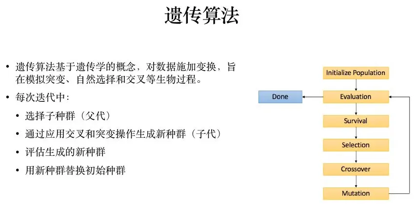
A basic GA repeats:

1. initialize a diverse population;
2. evaluate objective and constraint violation;
3. select parents;
4. recombine them by crossover;
5. mutate offspring;
6. preserve or select survivors;
7. stop under a declared budget or convergence rule.

Selection creates pressure toward strong candidates. Crossover reuses partial structure. Mutation introduces variation. Elitism protects the best known solution, but too much elitism collapses diversity.

Perform one generation by hand

Let us run a tiny evolutionary step with the bag. Start with two feasible parent chromosomes:for A+C, value twelve, andfor B+E, value seven. Cut both after the second bit. Written with a separator, the parents areand. Cross the left prefix of one with the right suffix of the other. The children are, which chooses A+E with value six and weight three, and, which chooses B+C with value thirteen and weight seven. One child is worse than either parent in value; the other improves on both. Crossover is not a guarantee of progress. It is a way to recombine pieces of candidate solutions and let evaluation determine which recombinations help.

Now mutate one bit of the weaker child: flip its C position from zero to one. The new child is, choosing A+C+E, weighing seven kilograms, and earning value fourteen—the exact optimum we found by enumeration. This is a lucky teaching run, not evidence that mutation usually finds the optimum in one step. Its job is to show what a flip means: an item is added or removed, and both capacity and value must be recalculated. In code, a mutation unit test can assert that exactly one position changed under a one-flip operator and that the chromosome still has five bits.

Which parents should be selected for the next generation? If we always keep only the current best string, we may lose the B+C combination or other building blocks that could matter when capacities or values change. If we keep every low-value string forever, selection pressure disappears. Survivor selection balances those forces. A small elite can preserve value fourteen as the best known feasible solution, while other slots keep distinct candidates. In this toy instance, once fourteen is found we know it is globally optimal because we already enumerated the space. In a large problem, an elite stores the best found; it does not turn the result into a proof of global optimality.

Now replace the second parent with an infeasible one,for B+C+E at weight eight and raw value fifteen. A selection method that sees only raw value might choose it over every feasible parent, encouraging the population to live outside the bag limit. We must either penalize its violation, repair it, or compare feasibility first. Each choice changes which genetic material is available to crossover. Constraint handling is therefore not a small after-the-fact cleanup step. It shapes the evolutionary path from the start.

The one-generation calculation also gives us a natural software audit. Record parents, cut position, child strings, weights, values, mutation position, repaired strings if any, and survivors for a fixed random seed. If the displayed parent isbut the evaluator says it weighs eight kilograms, the bug is in encoding or data order, not in the search strategy. If a child has six positions, the bug is in crossover. If a value-fifteen overweight string is reported as best feasible, the bug is in the feasibility test. A small trace can diagnose the method more clearly than a thousand-generation fitness plot.

Fitness and constraints

For maximization with violation, a penalty fitness may be

The penalty must be large enough to discourage infeasibility but not so large that the search receives no useful gradient toward the feasible region. Better alternatives include repair operators, feasible encodings, and feasibility-first comparison:

Penalize the overweight bag honestly

Our overweight stringselects B,C,E. Its raw value is fifteen, weight eight kilograms, and violation one kilogram. With penaltyvalue-points per excess kilogram, penalized fitness is. That is larger than the exact legal optimum’s fitness fourteen, so a selection procedure based solely on this number can prefer an illegal bag. With, its fitness is fourteen, tied with the optimum; depending on tie handling, it may still survive as if it were just as useful. With, its fitness is thirteen, below the optimum, but it can still beat several legal bags. The penalty is not “correct” just because we gave it a Greek letter. Its effect depends on the value scale, degree of violation, and which candidates the search has found.

Suppose another string weighs ten kilograms and has raw value twenty. A two-point-per-kilogram penalty gives fitness. It can again tie the legal optimum. A penalty large enough for one illegal candidate may not be sufficient for another. We might set a penalty from an upper bound on the value that extra weight can bring, use adaptive penalties, or avoid one scalar fitness comparison across legal and illegal candidates. Whatever we choose, the paper must report the best feasible objective separately from any penalized fitness. A fitness curve that climbs to twenty while all selected bags exceed capacity would be evidence of model failure, not progress.

Feasibility-first comparison gives a simple rule the field worker can understand: a legal bag beats every illegal one; between legal bags, choose higher value; between illegal bags, choose the smaller overweight amount. This rule does not require a value-to-kilogram exchange coefficient. It can be powerful when feasible bags are easy to construct, but if the initial population is entirely infeasible and violations are indistinguishable, the algorithm may have trouble reaching the legal region. Seed some legal candidates, or design a repair that moves illegal ones toward feasibility. We should test the feasible fraction each generation instead of assuming the ordering rule magically creates legal offspring.

Now repairby dropping one item. It exceeds capacity by one kilogram. If we drop E, the repaired bag is B+C, weight seven and value thirteen. If we drop B, it becomes C+E, weight five and value ten. A rule that always drops the item with the smallest value-to-weight ratio would drop B first because B’s ratio is, below E’s ratio. That rule repairs capacity but loses five value points, whereas dropping E loses only two. For this particular excess, “worst ratio” is not the same as “least lost value that restores legality.” If a domain repair always follows one ordering, it may funnel diverse offspring into the same few bags, lowering exploration. Document the rule and test its bias.

Constructing only legal subsets offers another route. Start with an empty bag, visit items in a chosen or randomized order, and add an item only if it fits. Every initialized bag is legal. But crossover and mutation can make it overweight again unless their own implementations preserve capacity or call repair. Also, fixed greedy construction may never initialize some useful low-density combination. A legal encoding solves one problem—invalid initial states—while possibly creating a different search bias. We evaluate both.

There is a modeling nuance worth repeating. If a researcher truly permits eight kilograms by paying for a stronger bag, the variable “rent extra capacity” and its cost should be inside the objective and constraints. In that new modelmight be legal and even attractive. A GA penalty is not a substitute for discussing whether capacity is flexible. We first decide what the field worker can actually do; then we design fitness to reflect that decision.

1. a feasible candidate beats an infeasible one;
2. among feasible candidates, compare objective;
3. among infeasible candidates, compare violation.

Operators must respect structure

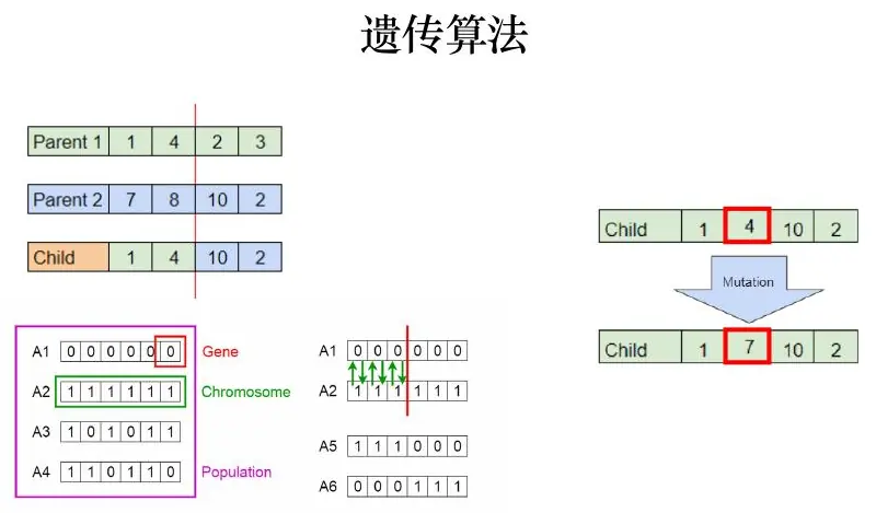
One-point crossover is natural for bit strings but can duplicate cities in a route. Permutation problems need order crossover, partially mapped crossover, or other structure-preserving operators. A mutation may flip a bit, swap two positions, reverse a route segment, or perturb a real coordinate.

The operator is part of the model. Explain why it produces meaningful nearby solutions.

A chromosome can be valid yet semantically broken

Our five-item bag has no ordering requirement; a bit flip adds or removes one item. A route is different. Imagine four cities at the corners of a unit square: A at, B at, C at, and D at. A tour must visit each city once and return to the start. A–B–C–D–A follows the square perimeter and has length four. A–C–B–D–A crosses diagonals and has length. In this tiny geometry, reversing part of the crossing tour can remove the crossing and improve distance. That is why an inversion or 2-opt-style move has meaning for routing: it changes edges in a way related to the physical objective.

Now take two perfectly valid parent permutations,and. Cut after two positions and use ordinary string crossover: the first parent’s prefixfollowed by the second parent’s suffixproduces. C and D have disappeared, while A and B occur twice. The child is not a poor tour; it is not a tour at all. If we score it by four route edges, we have changed the problem. A route-preserving operator must copy or repair cities so each appears once. Order crossover, partially mapped crossover, and edge recombination are different ways to do that, each with its own notion of useful inherited structure.

Suppose we use a repair that scans a child left to right and replaces each duplicate with the first missing city alphabetically. It restores permutation legality, but may add edges unrelated to either parent. If we instead preserve a parent edge set, the child may better inherit short local segments. We should compare these operators not by their names but by what they preserve: city membership, neighborhood edges, relative order, or long subsequences. A unit test checks exact city membership and uniqueness for every generated child; an experiment then checks whether the preserved structure improves distance under equal evaluation budgets.

This is not a claim that the GA is the best algorithm for the square or even for many larger tours. The square is exactly solvable by inspection. For modest tours, specialized integer programming, dynamic programming, 2-opt, or other routing heuristics may be faster and more reliable. We use the square as a microscope: it shows how a generic operator can produce an invalid object and how a meaningful neighborhood move relates to the geometry. When the tour grows, those lessons remain, even though we can no longer inspect every possible order.

The same failure can happen in a task schedule while every string still looks like a complete list. Suppose two workers may begin at either location A or B, travel between them takes thirty minutes, and tasks T1/T2 run 9:00–10:00 at A/B while T3/T4 run 10:00–11:00 at A/B. The legal assignment vectormeans worker 1 does T1 then T3 at A, and worker 2 does T2 then T4 at B. A second legal assignment swaps the worker labels throughout:. Cut and cross these vectors after two tasks. One childgives worker 2 T2 at B then T3 at A with zero travel time, and worker 1 T1 at A then T4 at B. Every task has a worker, but both workers must teleport at 10:00. The chromosome is syntactically complete and operationally infeasible.

We could repair the child by reassigning the later tasks, or encode task order and use a schedule decoder that checks travel and availability. But a decoder may fail to place all tasks or may systematically favor the first worker. Record the number of completed tasks, rejected tasks, and reasons. If a small exact assignment solver already handles this schedule, use it. A GA becomes appropriate only if the full problem has additional complexity that defeats the stronger structure or if a fair comparison shows the GA adds value. The phrase “genetic algorithm” is not a reason to discard an exact method.

Exploration versus exploitation

Population size, selection pressure, crossover rate, and mutation rate control the balance. Diagnose the search with:

• best and median fitness by generation;
• feasible fraction;
• population diversity;
• improvement versus objective evaluations;
• variation across random seeds.

If all candidates become identical early, increase diversity or reduce selection pressure. If fitness never improves, inspect encoding, repair, and scaling before increasing iterations.

The pressure dial is not just “keep the best”

Imagine a population of six legal bags with values. One possible parent-selection method is a tournament of two: randomly sample two candidates and select the better. If the sample is value twelve versus seven, twelve wins; if it is thirteen versus fourteen, fourteen wins. A tournament of six, by contrast, selects fourteen every time when all six are sampled. That strong pressure can cause every parent to be the same chromosome, after which crossover produces little new information. A tournament of one selects a random parent and supplies no value pressure. The choice of tournament size controls how quickly the population concentrates, and we can observe its consequences through uniqueness and diversity, not merely through the final score.

What is diversity in a bit-string population? A simple Hamming distance counts positions where two chromosomes differ. For instance,anddisagree at four of five positions, whileanddiffer only at E. Average pairwise Hamming distance gives a rough measure of spread. But high spread alone is not proof of useful exploration: a population of many infeasible strings can be diverse and still never pack a legal bag. Plot diversity beside feasible fraction and best feasible value. If diversity falls while feasible value stops improving, premature convergence is plausible. If diversity remains high but all candidates violate capacity, inspect constraint handling rather than increasing mutation blindly.

Elitism preserves the best known legal chromosome across a generation. Suppose we foundat value fourteen and random crossover makes only lower-value children. Keeping one elite ensures we do not forget fourteen. That is sensible. But if four of six slots are copies of the elite, many parent pairs are identical; their crossovers return the same string and consume evaluations. The aim is not to abolish elitism but to keep its amount proportional to the need for memory. For a large expensive problem, a small archive of distinct strong feasible candidates can be more useful than many clones of one winner.

Mutation has a probability interpretation often omitted from beginner summaries. A common bitwise choice is mutation probabilityfor a chromosome ofbits. It changes one bit on average, not exactly one bit every time. For our five-bit bag,. The probability that no bit flips is; the probability that exactly one flips is; the remaining probability, about, covers two or more flips. So “mutation rate 0.2” is not equivalent to the one-flip operation we performed by hand. If our implementation always flips exactly one bit, say that. If it independently tests every bit, report the per-bit probability. Such details change the neighborhood the GA explores and make results reproducible.

What happens when mutation is too aggressive? A carefully assembled bag can lose several good items at once; a route can be scrambled beyond useful inherited structure. When it is too timid, identical parents produce identical children and the search cannot recover from a narrow population. One can adapt the rate after a documented diversity drop, but that is another model component: define the threshold, upper rate, and whether it acts on all individuals or only non-elite ones. A plot of best value alone cannot show whether the mechanism worked. Track accepted mutations, unique offspring, feasible offspring, and improvements per evaluation.

This leads to a diagnostic order for the person running the experiment. If progress stops, first verify objective and constraint calculations on the five-item oracle. Then inspect the number of unique legal children after crossover and mutation. Then ask whether survivor selection is cloning too aggressively. Only after those checks tune population size or add generations. A broken evaluator run for twice as long remains broken. Tuning should respond to a measured mechanism, not to the feeling that the algorithm needs a larger number.

Evidence for a competition paper

Compare the GA with an exact solver on small instances and with a simple heuristic on full instances. Report computational budget, number of runs, median outcome, best outcome, and variability. A single lucky run is not evidence.

Use the GA only after asking whether the model has exploitable structure. Linear assignment, shortest path, convex quadratic programming, and many scheduling models have specialized solvers with stronger guarantees.

Decide what the GA has to beat

For the five-item bag, enumeration produces value fourteen as an exact optimum. A MILP can also express the additive bag objective and capacity rule with binary variables. SciPy’s official milp interface supports linear constraints and integrality and reports a solver status and mixed-integer gap (documentation ). For five items this is overkill, but the comparison is instructive: if a conventional integer solver handles the real-size formulation within the deadline, why should we accept a stochastic method with no optimality certificate? The GA may still be useful for a nonlinear black-box objective or a difficult custom schedule, but that is a reason about structure, not a preference for an exciting algorithm name.

When the exact method cannot finish on a large case, retain a small exact case as a software check. Create a miniature problem with known optimum, then increase size while preserving the same rules. The miniature tells us whether the GA can navigate the model at all. On the large case, compare with at least one simple feasible heuristic that a practitioner could actually use. For a bag, sort items by a declared value-to-weight rule, add what fits, and perhaps perform a swap-improvement pass. For a route, start with nearest-neighbor and improve crossings with 2-opt. For a schedule, assign tasks earliest-deadline-first while checking travel and resources. These are not straw men. A GA that needs a thousand evaluations to match a five-minute local heuristic has not earned its complexity.

Measure the same objective on the same legal problem. If a GA reports raw value twenty from an overweight bag while the heuristic reports legal value thirteen, comparing twenty with thirteen would reward constraint violation. If one route method includes the return edge and another stops at the last city, comparing their lengths is meaningless. If one schedule counts incomplete tasks and another requires all tasks to be performed, they are optimizing different outcomes. A fair comparison starts by putting each returned candidate through the same independent feasibility and objective function.

Equal budgets reveal mechanisms

Suppose GA configuration A initializes twenty candidates and produces twenty new candidates in each of fifty generations. It proposes roughlyobjective evaluations. Configuration B initializes one hundred candidates and produces one hundred in each of fifty generations, proposing aboutevaluations. A comparison at “fifty generations each” gives B five times the chance to search, so its better result would not isolate a better mechanism. Use evaluation count or wall-clock time as a common horizontal axis. If objective evaluation is a costly simulation, both can matter: one method may produce candidates rapidly but spend time repairing them, while another spends little repair time and more simulation time.

Keep a record of unique evaluated candidates too. In the five-item problem, there are only 32 strings. A GA proposing thousands of strings must revisit many. We can cache the weight and value of identical legal strings to avoid unnecessary recomputation; however, the number of candidate proposals and unique evaluations should then both be reported so readers know how the budget was spent. If each evaluation includes new simulation randomness, caching a single noisy score would be a different assumption and could be dangerous. Define what one evaluation means.

Across independent random seeds, summarize median outcome, spread, best and worst feasible outcomes, feasibility rate, and the fraction of runs that match the small-case oracle when one exists. A “best of thirty runs” result tells us what is possible after thirty attempts, not what a typical user gets from one attempt. Suppose a hypothetical thirty-seed test on the five-item bag found value fourteen in eighteen runs and thirteen in twelve. The best is fourteen, the median is fourteen, and the success frequency is 60%. Reporting only the best hides the twelve runs that missed a tiny exact optimum. This is an illustrative data-reading exercise, not a claim that we ran such an experiment for the site. A real paper should replace it with actual seed-level outputs and the precise configuration.

Plot best-feasible value against evaluations for each run, then perhaps a median curve with a spread band. If the band remains wide near the budget limit, the method is unreliable or budget-sensitive. If all runs flatten at the same value below the exact small-instance optimum, inspect operators and feasible-space access. If one run suddenly improves at a very late evaluation, a fixed shorter budget could have missed it. The curve explains the process, whereas a final average alone can hide how and when progress occurred.

The same evaluation discipline carries into the next lesson’s particle and annealing methods. We will not compare a GA’s 5000 objective calls with an annealing run’s 500 and declare a winner. We will compare equal budgets, seeds, legal objectives, and a known small oracle. The methods differ in how they move through space, but the evidence rules should stay the same.

The official SciPy optimization guide groups global optimizers by supported bounds, nonlinear constraints, and derivative requirements; solver choice should follow the mathematical structure of the problem (optimization guide ).

Minimal pseudocode

population <- create_feasible_candidates()
evaluate(population)

repeat until evaluation_budget_is_used:
    parents   <- select(population)
    offspring <- crossover(parents)
    offspring <- mutate(offspring)
    offspring <- repair_or_measure_violation(offspring)
    evaluate(offspring)
    population <- survivor_selection(population, offspring)

return best_feasible_candidate_seen

Keep evaluation count—not only generation count—because population sizes may differ. Cache repeated candidates when objective evaluation is expensive. For a beginner implementation, first test the loop on a function with a known optimum, then on a tiny version of the real problem whose exact optimum can be enumerated.

Read the pseudocode as a set of promises

The first line, create_feasible_candidates(), promises that we can generate legal starting points. For the five-item bag, we can start with empty strings, add items while weight stays at most seven, and independently check every generated string. If the task schedule is more complex, initialization may call a greedy decoder and keep only schedules satisfying time and travel rules. If creating any legal candidate is difficult, that is a warning about the representation or model, not a reason to silently begin with impossible plans.

The evaluate line must return at least objective value and a separate violation report. For the bag it can calculate weight and value directly; for the route it calculates every edge including the return edge and checks city membership; for the worker schedule it checks assignments, timing, travel, and conflicts. A single scalar fitness may be used inside parent selection, but the log should retain those components. Otherwise a later analyst cannot tell whether high fitness came from a good legal plan or from a permissive penalty.

The select line says which current candidates become parents, not which candidates survive forever. The crossover and mutate lines say how candidate information changes. The repair or violation line says how we restore or rank feasibility. The final survivor-selection line decides which parents and children remain in the population. These are separate decisions. A beginner implementation that overwrites parents with all offspring every generation may accidentally lose the best feasible bag; one that copies all parents and adds all children may grow population without bound. State population size and elite rule so the loop is actually defined.

The return statement says best feasible candidate seen, not “candidate with highest penalized fitness” and not “last candidate in the final generation.” In the bag example, we might temporarily see overweight raw value fifteen while our best legal value is fourteen. The algorithm must return the value-fourteen legal string. If we have only seen legal value thirteen, return thirteen with its weight and a clear statement that fourteen was the exact toy benchmark not found by this run. In a large problem without exact proof, report “best found” or a gap to a valid bound when one exists, never an invented optimality certificate.

Now imagine that evaluating a schedule involves a noisy simulation of customer arrivals. One schedule has true long-run average wait around ten minutes and another around twelve, but one unlucky sample gives them estimated waits of fifteen and seven. If we let the GA select on those two single draws, it may choose the worse schedule because its simulation happened to be lucky. Re-evaluate promising candidates on multiple scenarios and, when comparing two candidates, use the same arrival realizations for both where appropriate. This is called common random numbers: it reduces irrelevant differences caused only by different simulated days. Hold back independent scenarios for final validation so the GA cannot simply learn the peculiarities of the scenarios it repeatedly saw.

This is a form of overfitting, even though we are doing optimization rather than conventional prediction. A GA that tries thousands of schedules against the same ten arrival scenarios may discover a schedule perfectly adapted to those ten days but poor on new ones. Increasing the population or number of generations can make this worse if the evaluation sample stays fixed. The remedy is not to call the search “robust” because it is stochastic. Use a training scenario set for search, a separate validation set for model and parameter selection, and a final held-out set or stress scenarios for the recommendation. State which data each decision used and whether new information would have been available when the real schedule was made.

Separate random streams can help. The GA has randomness for initialization, parent choice, crossover points, and mutation. The simulator has randomness for arrivals or service times. If one seed controls everything, changing the population size may also change the simulated arrival sequence, making mechanism comparisons noisy. Record a search seed and a scenario seed separately, plus the data version and objective code version. Reproducibility is not merely writing “seed 42” in a caption; it is making clear what the seed governs.

When should the loop stop? A fixed objective-evaluation budget gives a fair comparison with other methods. An early-stop rule after many evaluations without improvement can save time, but it needs a threshold and can stop a method just before a late improvement. A known target value on the small oracle can terminate immediately once reached. A diversity-triggered restart can be useful when the population collapses, but the restart itself uses evaluations and must be counted. We should decide these rules before looking at the final curve, or a tuned stopping rule could be chosen to flatter one run.

Finally, let a colleague rerun one seed and inspect the per-generation record: number of candidates proposed, unique candidates, legal fraction, best legal objective, median legal objective, average violation of illegal candidates, and runtime. That record tells a coherent search story. A line chart of “fitness” alone may rise while real feasibility falls. Our implementation promises to make each step of the algorithm visible enough to challenge, because the model’s result will ultimately be a decision someone has to trust.

Practice

For a ten-item knapsack, compare three constraint strategies: penalty, repair by removing low value-to-weight items, and feasibility-first selection. Across 30 seeds, report feasibility rate, median objective, best objective, and evaluations. This exercise shows that representation and constraint handling matter at least as much as the word “genetic.”

The steps of a genetic algorithm are easy to memorize and easy to misuse. This workshop turns them into a tested procedure: a hand-checkable candidate, a feasible mutation, a baseline, and repeated runs that reveal variability.

Design a GA that can be trusted

Consider a traveling-salesperson problem with citiesand distance matrix. A candidate is a permutation, and its cost is

Choose representation before operators

A binary chromosome is unnatural here because most bit strings do not describe valid tours. A permutation representation makes feasibility automatic, but ordinary one-point crossover produces duplicated and missing cities. Use order crossover, partially matched crossover, or edge recombination. Swap, insertion, inversion, and 2-opt moves preserve permutation structure.

Representation controls the neighborhood the algorithm can explore. Inversion is especially meaningful for routes because it removes crossing edges. A domain-aware operator is not cheating; it is the difference between searching the problem and searching an arbitrary encoding.

Follow the square tour through a route improvement

We can make the route improvement exact. Start from A–C–B–D–A on the unit-square coordinates introduced earlier. The two diagonal edges A–C and B–D have lengtheach. The other two edges C–B and D–A have length one each, so total length is. A 2-opt move cuts two edges and reconnects the tour without duplicating a city. Cut A–C and B–D; reconnect A–B and C–D. The resulting cyclic order A–B–C–D–A has four sides of length one, total four. We saved aboutdistance units. We did not need a biological metaphor to explain why this move helps: crossing Euclidean edges are often a visible opportunity for a shorter uncrossed route.

Why not simply apply 2-opt to every route and stop? In this four-city case, that is enough. In a large tour, 2-opt can settle in a local optimum; different starting orders may lead to different final lengths. A GA could use a population of different tours, route-preserving recombination, and 2-opt as a local improvement step on offspring. That hybrid is often called a memetic algorithm. But if the hybrid performs thousands of 2-opt edge checks while the baseline performs only one pass, comparing only final route lengths would be unfair. Count distance evaluations or wall time, and include repeated 2-opt from several starts as a strong baseline. The GA’s population only earns credit for improvement beyond the effort we could spend on local search alone.

There is a reason the number of possible tours grows so fast. Fordistinct cities, a route order haswritten permutations, but many represent the same cyclic tour because choosing a different starting city does not change the edges. For a symmetric distance matrix, reversing the route also gives the same length. With a fixed start, there aredistinct undirected cycles. At twenty cities this is already about, far too many to check one by one in an ordinary course assignment. If roads are one-way and, reversal is no longer equivalent; we should not divide by two. The counting argument explains why heuristic search may be useful while also reminding us that the exact formulation and distance data matter.

What does a route chromosome mean when travel times change by hour? A permutation alone chooses the visit order, but it does not specify departure time, waiting, vehicle capacity, or time windows. The decoder must turn the order into a feasible schedule, perhaps inserting waiting or rejecting late visits. If a route arrives at a customer after their window closes, a short geometric path may not be a legal solution. A penalty for lateness may be appropriate only when lateness is actually permitted with a defined cost. If closing time is hard, feasibility-first comparison or a repair that changes visit order may be safer. The same questions we asked of a seven-kilogram bag now reappear as time, distance, and service rules.

An operator’s effect depends on those rules. A simple inversion preserves every city, but it can change arrival times for many later cities. A local edge improvement in distance may worsen a time-window violation. An edge-preserving crossover may retain good distance segments but move a heavy customer to a route where vehicle capacity is exceeded. We should evaluate the full candidate after every operation. “Structure-preserving” has to name which structure: city uniqueness is not the same as capacity, travel time, or appointment feasibility. In a paper, a small table of operator properties and observed feasible-offspring rates can communicate that better than a list of operator names.

The square example gives us a compact baseline story to tell a first-time reader. Ordinary one-point crossover fails city uniqueness. A permutation-aware crossover fixes that first problem. Inversion can remove a crossing and improve length. A route decoder adds time-window and capacity meaning. Repeated runs and equal-budget baselines then test whether the whole GA searches more effectively than local moves. Each stage solves a problem introduced by the preceding stage. That is why the route case belongs after the bag: it is not a separate algorithm parade, but a harder candidate representation with the same modeling discipline.

Separate selection, variation, and survival

Tournament selection controls pressure through tournament size. Crossover combines information, mutation restores local diversity, and survivor selection decides whether parents can remain. Preserve a small elite, but do not let elites occupy most of the population. Track the best, median, and worst cost plus the number of unique candidates. A falling diversity curve can warn of premature convergence before the best-cost curve becomes flat.

Fitness transformations should preserve ordering without creating numerical explosions. For minimization, avoidwhencan be near zero or negative. Tournament selection can use objective comparisons directly. With constraint violations, compare feasible solutions before infeasible ones and rank infeasible candidates by violation, or design a repair with a documented bias.

Decode a worker schedule instead of trusting labels

The two-location schedule we used earlier gives a simple decoder to imagine. A chromosome could be a priority order of tasks rather than a vector of worker numbers. For each task in that order, the decoder considers workers who are free throughout the task, can travel from their previous location before the start time, and have any required certification. It assigns the task to the worker whose choice causes the least extra travel or leaves the most future capacity, under a rule we have stated. If no worker passes, it records the task as unplaced rather than manufacturing a worker label. The decoded timetable—not the priority string itself—is the candidate decision we score.

Run that mentally on T1 at A 9:00–10:00, T2 at B 9:00–10:00, T3 at A 10:00–11:00, and T4 at B 10:00–11:00. If workers may begin at either location, a sensible decoder can give T1/T3 to worker 1 and T2/T4 to worker 2, completing four tasks with no cross-location travel. The chromosomeis only one way to request that schedule. A different priority order may decode to the same timetable, so many chromosomes can represent one physical solution. If the GA repeatedly evaluates those duplicates, caching by raw chromosome will not detect all repeated decoded decisions; caching by normalized timetable may.

Now insert a fifth task T5 at A from 9:30–10:30, worth a higher score than T1 alone but overlapping it and T3. A priority-first decoder may place T5 on one worker, T2 on the other, and then find T3/T4 impossible or possible depending on worker-location and end-time rules. A different order that starts with T1 and T2 may fill the morning in a way that leaves T5 out but makes later tasks possible. The value of a priority order therefore depends on the decoding rule, task rewards, and conflicts. We cannot call a chromosome “better” until we decode it and check the whole timetable.

What if a task is mandatory rather than optional? Then a decoder that leaves it out is not merely lower-scoring; it is infeasible. We may initialize only orders that decode to complete legal schedules, repair incomplete ones, or use an exact assignment model for that mandatory core and let the GA adjust optional tasks. A hybrid can be sensible: exact constraints protect indispensable assignments while evolutionary variation explores uncertain or irregular optional choices. But the hybrid’s exact solve time belongs in the method’s total budget. The practitioner should see which guarantee came from the exact part and which outcome is only best-found by the GA.

This is also where the user-facing decision matters more than the genetic story. If the decoded schedule sends a worker between A and B without the required thirty minutes, reject it. If a worker has only a ten-minute gap and travel needs thirty, no mutation-rate adjustment will make the schedule physically real. If the exact four-task baseline already completes everything, a GA that also completes four has not improved task count. It might reduce travel or improve robustness, but that secondary objective must be named and fairly evaluated. A strong modeling article follows the actual people and clocks through the decoder, not just the colorful chromosome picture.

Budget comparisons fairly

If population size isand the algorithm runsgenerations, it uses roughlyobjective evaluations. Compare methods at the same evaluation or wall-clock budget. Run independent seeds and report median, interquartile range, best, and feasibility rate. Use paired seeds or common test instances when comparing configurations.

On small, enumerate or solve exactly to measure optimality gap:

On large instances, compare with nearest-neighbor and repeated 2-opt baselines. A GA that cannot beat a simple local search is not justified.

Tune mechanisms, not a magic list

Use pilot experiments to study population size, mutation probability, tournament size, and elitism. Change one mechanism at a time or use a designed experiment. High mutation makes the search nearly random; very low mutation may prevent recovery after convergence. Adaptive mutation can increase variation when diversity falls, but its trigger and limit must be stated.

Practice

Implement a permutation GA for 20 cities. Unit-test every operator for length, uniqueness, and city membership. Plot objective and diversity by evaluation count. Compare order crossover with edge recombination and swap mutation with inversion. Run 30 seeds, compare against nearest-neighbor plus 2-opt, and explain performance using the structure each operator preserves.

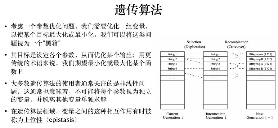
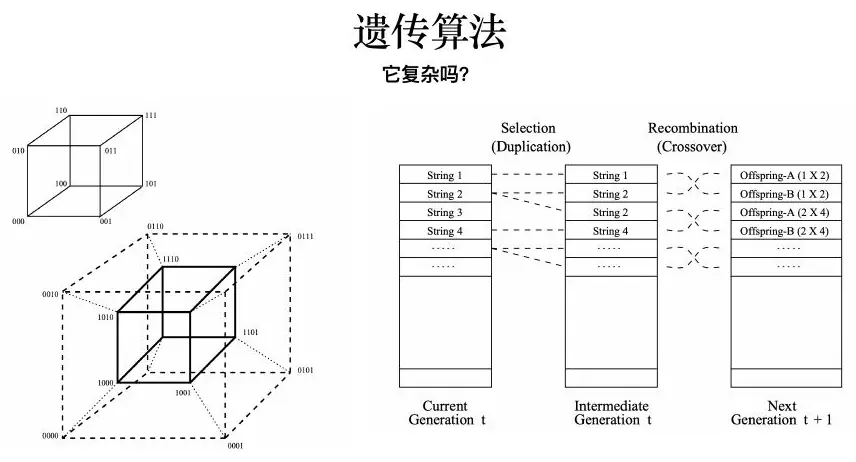
Our workshop treated operators as design choices. The lecture’s own sequence shows how encoding, population updates, constraint handling, and stopping checks fit together in one search narrative.

The lecture’s complete evolutionary story

Selection creates pressure; variation creates candidates; evaluation connects them to the model.

Operators should preserve useful building blocks without destroying diversity.

Knapsack makes encoding, feasibility, penalty, and repair concrete.

Epistasis means one gene's value depends on others; independent tuning can fail.

Binary, real-valued, and permutation encodings induce different neighborhoods.

Why the genes may not be independent

The slide’s term epistasis comes from genetics, but here we can translate it into an ordinary planning problem: the benefit or feasibility of one decision depends on another decision. Let C in our kit be a camera and E a battery. Suppose the camera cannot be used unless the battery is packed. Then add the hard rule. Under the original weight-only bag model, B+C at value thirteen was legal. Under this new dependency, B+C without E is no longer a usable kit. A+C+E at value fourteen remains legal. We changed the problem, so we must update the exact small-instance oracle as well as the GA fitness. The previous optimum happens to remain the same, but we cannot assume that for every new rule.

The gene interaction can also affect value rather than feasibility. Suppose packing A and C together adds three units of research value because A is a calibration plate and C is a camera that can use it. Then value is. The extra benefit appears only when both bits are one. A one-item value-to-weight ranking cannot see that synergy; crossover that separates A from C may lose more than the sum of their individual scores suggests. This is the modeling meaning of epistasis. It is not proof that biology-inspired search is uniquely required. We could linearize the two-bit product with a helper binarysatisfying,, and, then putin a mixed-integer objective. For a small or structured instance an exact MILP may still be preferable.

Now ask how chromosome order interacts with the camera-battery rule. If C and E are far apart in the bit string, one-point crossover may often inherit C without E, creating a child we must reject or repair. If they are adjacent, some cuts preserve the pair more often. But grouping one pair may separate another useful pair. We can use a feasibility-aware operator that copies required companions, a decoder that adds batteries when cameras are selected, or a repair that removes cameras without batteries. Each method has costs and biases: automatically adding E consumes capacity, while automatically dropping C may lose high-value opportunities. The operator design should match the dependency structure we actually declared.

The original overweight B+C+E bag now gives us a repair puzzle with that dependency. It weighs eight kilograms, exceeding capacity by one. If C really requires E, dropping E is no longer a valid repair: B+C would weigh seven but leave the camera without power. Dropping B yields C+E, which weighs five and has value ten. Dropping C yields B+E, which weighs four and has value seven. So the best one-item deletion among these usable repairs is dropping B, even though it loses more raw value than dropping E in the earlier base problem. A repair rule must respect all constraints, not just the capacity constraint it happened to notice first.

What if C and E can share one battery with another device, or E has enough charge for only a certain number of operations? A simple implicationmight no longer capture the rule. We may need battery capacity, energy consumption, or operating-time constraints. The GA cannot detect that missing physics. The example is deliberately small so a reader can see the progression: first weight, then companion requirement, then a possible quantitative resource limit. Each extension changes which offspring are useful and which repairs are lawful.

The bonus-value example has a similar effect. If A+C together earn three extra points, removing A or C from a bag loses both the individual’s points and the synergy. A repair ranking based only on each item’s individual value-to-weight ratio underestimates that loss. We could compute the marginal value lost by deletion from the current bag, including interaction terms, and choose a deletion that restores feasibility with least total lost value. That local calculation may still miss a better multi-item swap, but it respects the current objective more closely than a static item ranking. Domain-aware repair can be powerful; it also requires the objective and constraints to be genuinely specified.

This is why the lecture’s epistasis slide belongs next to the operator discussion. Interaction is not a mysterious property that merely makes a problem “hard.” It tells us which candidate parts must be interpreted together. Selection on raw independent scores, crossover across a required pair, or repair based on isolated ratios can all fail for the same reason. Once we can name the dependency in ordinary language, we can test whether an exact formulation, a tailored GA operator, or a different encoding handles it best.

The same phenomenon in the worker schedule is travel time: assigning T3 to worker 2 may be harmless if that worker just finished a task at A, but impossible if they just finished at B. The “value” of one assignment bit depends on previous task bits. This is why a raw vector of worker labels can be a poor GA chromosome for travel-constrained scheduling. A route-order encoding or a legal decoder may preserve more meaning. Once again, representation is not decoration; it decides which relationships the search can easily keep.

A small black-box parameter problem

The lecture slides also talk about setting several parameters of a black-box system to maximize or minimize an output. We can make that idea concrete with a bakery conveyor. Suppose a tray passes through a heating zone. We can choose conveyor speed, low or high, and heater setting, low or high. The bake-quality score is measured after the batch, so for now imagine we only have the following illustrative pilot results, not a clean physical equation:

Conveyor speed	Low heater quality (%)	High heater quality (%)
Low	70	92
High	60	75

At low speed, raising heater setting improves the quality score by 22 percentage points. At high speed, it improves by only 15 points. The effect of heater setting depends on conveyor speed; the settings interact. If a student tunes heater only at low speed and then assumes the same improvement at high speed, they are extrapolating a relationship the pilot table does not support. This is the black-box meaning of epistasis in a parameter model. We are not required to call the system biological; we only need to see that decisions cannot necessarily be separated into independent one-variable optimizations.

But would we run a GA for this two-by-two table? No. Evaluate all four legal combinations. The highest observed quality is 92% at low speed and high heater, under the pilot conditions. We must still check throughput and energy. If low conveyor speed processes only half as many trays per hour, a manager might prefer a faster setting with 75% quality, or might require quality at least 90%, ruling it out. One quality number is not a complete decision objective. The GA does not repair missing throughput, energy, or acceptance constraints; these belong in the model first.

Now imagine ten continuous settings: belt speed, zone temperatures, airflow, humidity, recipe dwell time, and several robot-arm timing parameters. A high-fidelity simulation or physical pilot yields the quality and throughput only after evaluating a full parameter vector. Derivatives may be unavailable, simulation may have local peaks, and evaluations may be expensive. A real-valued GA could search bounded vectors, using arithmetic or blend crossover and bounded perturbations instead of bit flips. Yet we should first test a designed experiment, local search from several starts, or a surrogate model. The reason for a GA would be a difficult black-box landscape under a finite evaluation budget, not merely the fact that ten parameters interact.

Bounds matter for real encodings just as capacity mattered for the bag. If temperature is safe only betweenand, a mutation that adds noise must clip, reflect, resample, or otherwise handle an out-of-range value. Each boundary rule biases search differently: clipping piles candidates on the bound, reflection keeps step magnitude but changes direction, resampling changes the mutation distribution. If a physical experiment is being performed, illegal parameter settings can damage equipment. We cannot let an optimizer “explore” unsafe temperatures just because their scores are assigned a penalty afterward.

There is measurement noise as well. One tray at a setting can bake well by chance because dough thickness varies. Repeat pilot conditions, randomize the order of trials, and compare settings on a common batch or controlled covariates when possible. A GA searching physical experiments can overfit incidental pilot noise, especially when it tests many vectors and celebrates the single highest observed score. Hold back confirmatory runs for finalists. Optimization of a black box is also experimental design: the search algorithm and the evidence about quality cannot be separated.

So the parameter case completes the slide’s evolutionary story. An encoding defines what a setting is; evaluation returns a quality and a safety report; crossover and mutation create new settings; interaction means whole vectors matter; and repeated controlled measurements decide whether a “best found” setting is actually better. The bakery is a new teaching illustration, not a claim that the course slides contained these numbers. It shows how to transfer the lecture’s abstract black-box idea to a situation a beginner can picture.

Knapsack from chromosome to fitness

For values, weights, capacity, chromosomerepresents a subset:

Penalty fitnessis simple but sensitive to. Repair can remove low value-to-weight items until feasible. Feasibility-preserving construction samples only legal subsets. Compare these mechanisms by feasible-offspring rate and best feasible objective.

Tournament size controls selection pressure. One-point crossover suits ordered strings but is arbitrary for unordered items; uniform crossover treats positions symmetrically. Bit mutation nearchanges one bit on average. Elitism preserves the best candidate but excessive elitism collapses diversity.

For continuous variables, use real-valued crossover and Gaussian or polynomial mutation. For routes, use order or edge-preserving crossover and swap, insertion, or inversion mutation. Ordinary one-point crossover creates missing and duplicate cities.

Evidence, not one lucky run

Plot best and median feasible objective versus evaluations, diversity versus evaluations, and final values across 20–30 seeds. Compare with exact optima on small cases and greedy/local baselines on large cases. Fix the number of objective evaluations, not generations, across algorithms.

The best bag can stop being legal tomorrow

We found A+C+E at value fourteen with capacity seven kilograms. Suppose the weight of E was estimated as one kilogram but the packed version actually weighs two. The old chosen bag now weighskilograms and violates the seven-kilogram limit. Re-enumerating the five-item base problem with E at two kilograms gives a new exact maximum of thirteen, achieved by A+D or B+C at weight seven. The value-fourteen solution did not become “slightly less good”; it became unusable under a hard limit. A one-kilogram input correction changed the decision set. The GA can be rerun, but the crucial modeling response is to update the item data and the feasibility test, then explain the changed recommendation.

Suppose instead the bag’s permitted capacity is uncertain: it will be seven kilograms on a normal trip but only six on a flight with a stricter allowance. If the kit must be legal on both trips and we cannot repack, use capacity six in the hard constraint. Under the original item weights, A+C has weight six and value twelve, the best legal fixed bag for that stricter allowance. We have given up two value points compared with the seven-kilogram optimum for a specific protection. If we can repack after seeing which trip occurs, a two-stage policy could choose A+C+E for the seven-kilogram trip and A+C for the six-kilogram trip. Again, the question is decision timing. The GA is a search tool for whichever formulation we choose; it is not itself a theory of uncertainty.

This makes the reported result more useful. A paper might say, “For the declared seven-kilogram kit and item scores, the best feasible chromosome found was A+C+E with value fourteen; enumeration of the five-item check confirms it is optimal in that toy instance. Under a six-kilogram capacity the best fixed kit is A+C with value twelve. The proposed larger-instance GA has no global-optimality certificate, so its reported value is best-found after the specified evaluation budget and thirty independent seeds.” That sentence separates the exact small oracle, sensitivity, and heuristic large result. It does not borrow a guarantee from one setting and apply it to another.

If we also adopt the later camera-battery dependency, the six-kilogram A+C kit may no longer be legal because C requires E. We would then solve the extended problem anew. Keeping the same sensitivity table while quietly changing rules would be a mistake. This is why example versions matter: original weights and only capacity; revised E weight; revised capacity; added dependency. Each version has its own feasible set and optimum. A traceable result table names its rule version, not just a chromosome string.

What the algorithm cannot discover for us

A GA can explore a huge space of encoded candidates. It cannot decide whether item values are comparable, whether a battery is mandatory for a camera, or whether a worker can teleport between tasks. Those are domain statements. It cannot infer from a low penalty score that an overweight bag is physically acceptable. It cannot convert thirty stochastic runs into a proof that the chosen tour is globally shortest. It cannot validate a bakery temperature recommendation if the quality scores came from one noisy tray per setting. These limits are not reasons to avoid GA entirely. They are reasons to place it inside a modeling process that has defined decisions, data, rules, baselines, and checks.

The lecture’s biological metaphor is useful for remembering the loop: candidate population, selection, recombination, mutation, evaluation, replacement. We should not stretch the metaphor beyond that. A chromosome is a coding choice, not a literal organism. A crossover operator is a way to build new candidate solutions, not a guarantee of inherited excellence. “Evolution” here means repeated selection under our chosen fitness and constraints, not natural selection toward a universally good schedule. When a beginner understands the physical candidate behind each gene, the metaphor supports rather than replaces reasoning.

Imagine a teammate asks why the route GA beat a nearest-neighbor baseline on some instances but not others. A weak answer is, “Random search sometimes gets lucky.” A stronger answer would inspect which instances contain crossing edges, tight time windows, or clusters; whether inversion removes crossings; whether the route decoder rejects offspring near windows; and how often the GA population retains distinct tours. If GA improvement concentrates on clustered tours after edge-preserving crossover, we have a mechanism to investigate. If it vanishes when both methods receive equal 2-opt effort, the apparent GA advantage may have come from local search budget rather than population search. The evaluation should tell us why the result changed.

For the bakery black box, a teammate might ask why quality reached 92% in the pilot but only 85% in confirmation. We should inspect batch variability, sensor calibration, search overfitting to repeated pilot evaluations, and whether the heater setting changed actual tray temperature. The GA’s numeric settings are not the conclusion until an independent trial confirms their effect. If the high-quality condition violates energy or throughput constraints, the candidate is not operationally best even if quality is measured accurately. The result has to travel from algorithm score back to a real action.

For the worker schedule, a teammate might ask why a candidate with four assigned task labels completed only three tasks in practice. Follow the decoded timetable: a travel delay, overlapping task, or missed preparation window can invalidate one label. A schedule chromosome and a schedule execution are different objects. Verify the decoder, stress travel times, and show which tasks survive. This is the same “small counterexample first” habit from our first modeling lesson, now applied to a more sophisticated search method.

The final communication should therefore be about choices, not only chromosomes. For the kit, list selected items, total weight, value, and capacity margin. For a tour, show visit order, length, return edge, window and capacity status, and comparison with a simple feasible route. For a schedule, show actual worker timelines and conflicts checked. For parameters, show physical settings, quality uncertainty, throughput, safety bounds, and confirmation data. A chromosome code can appear in an appendix for reproducibility; the main text should let a reader see the decision it represents.

When we move to particle swarm and simulated annealing, this modeling frame stays intact. Their motion rules are different: one method shares promising positions across a population; another sometimes accepts a worse local move to escape a narrow basin. But both will still need a lawful candidate representation, a meaningful objective, equal-budget baselines, repeated runs, and a story about when an output becomes an actionable decision. That continuity is more important than memorizing three separate lists of algorithm steps.

Genetic search gives us one way to explore difficult spaces, but its results depend on encoding, operators, constraints, and fair comparisons. The next lesson contrasts that population logic with particle motion and annealed local moves.
Keep the five-item instance in the test suite when implementing a larger GA. Its known legal optimum and intentionally illegal high-value string make changes in fitness, repair, or bit ordering immediately visible. A new algorithm curve is worth interpreting only after those basic meanings still pass.