Mathematical Modeling 7 - Trade-offs and Uncertainty

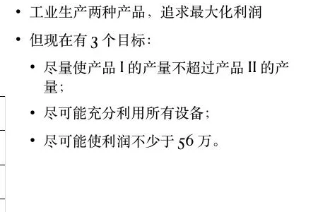
The factory from the optimization lesson may maximize profit and still disappoint its manager. Perhaps product I should not outnumber product II, idle equipment should be avoided, and profit should remain above a target. Can one solution satisfy all three wishes, and what happens when they conflict? Try ranking those wishes yourself before we assign any weights.

This lesson will separate two difficulties that are often blurred together. Multiple objectives ask whose priorities govern the choice; uncertainty asks what happens if prices, demand, or capacity forecasts are wrong. We will use small production choices to make Pareto trade-offs visible, then compare weighted, goal-based, robust, and scenario approaches. At the end, you should be able to explain why a recommendation is reasonable without pretending it is best under every preference and every future.

Real decisions rarely have one objective and perfectly known inputs. Profit competes with risk, service with cost, and nominal efficiency with resilience.

Start with separate objectives

Letmeasure the competing goals. Before combining them, solve each single-objective problem. These anchor solutions reveal scale and conflict: how much service is sacrificed by the cheapest plan, and how much cost is required by the best service plan?

A solutionis Pareto efficient if no feasible alternative improves one objective without worsening another. The Pareto frontier is therefore a map of defensible trade-offs, not a single automatic answer.

First solve the questions one at a time

In the production slide, “make the most profit” givesand 620,000 yuan. “Never make more I than II, then make the most profit” gives the continuous balanced planand 600,000 yuan. “Use all machine time” is not by itself a full objective: many combinations satisfy, including both of those plans. So we should not ask a solver for a unique “equipment optimum” without saying what breaks ties. The anchoring exercise exposes exactly this difference between a score to optimize and a target that can be met by many plans.

What is the actual conflict? The profit maximum violates balance by one unit of product. The balanced continuous maximum sacrifices two units of the slide’s profit scale, or 20,000 yuan, while leaving one kilogram of material unused. Both fill all ten machine-hours. So equipment utilization is not the source of this particular conflict; balance and nominal profit are. That statement is already more useful than announcing that a “multiobjective problem” exists. It tells the manager which two wishes they must discuss.

If the material capacity were much lower, equipment use might become another conflict. Suppose the factory receives only eight kilograms, with the same machine capacity. It may be impossible to use all ten machine-hours under some production ratios while also meeting the profit target. We would check feasibility before assigning penalties. A target that is reachable in the original data may become unreachable after a resource change. The manager should see which new fact created the conflict, not be told that the algorithm “struggled.”

To form a Pareto comparison, list each candidate with all outcomes. For: profit 62, excess-I imbalance 1, idle machine-hours 0, material use 11. For: profit 60, imbalance 0, idle machine-hours 0, material use 10. Neither dominates the other on profit and imbalance: the first is richer, the second fairer. For: profit 54, imbalance 0, idle machine-hours 1, material use 9. The balancedplan is no worse in balance and better in profit and machine use, so it dominatesin the continuous model. But if units must be whole, the fractional balanced plan is not legal and cannot dominate a legal integer plan. Pareto claims depend on the feasible set and variable domains.

Weighted sums

The common scalarization

requires normalized objectives. Without normalization, units decide the result. Weights encode preferences; they are not empirical facts.

Weighted sums can miss non-convex parts of a Pareto frontier. They are still useful for convex models and for sensitivity sweeps over multiple weight vectors.

What a weight actually says

Imagine a cost objective in dollars and a shortage objective in MWh. If we write, the numeral one beside shortage implicitly says that one MWh of shortage is worth one dollar of cost. That is probably not what anyone intended; we just allowed units to choose the preference. If we normalize both scores to comparable ranges, we can at least ask a stakeholder how much a movement across the observed cost range matters relative to a movement across the shortage range. Even after normalization, the weight is a choice, not a quantity estimated from the electricity data.

The city table makes the preference visible. Going from 70/30 to 50/50 saves 800 dollars and raises calm shortage by 20 MWh. If the manager uses a simple shortage penalty of 30 dollars per MWh in the calm scenario, the extra modeled penalty is 600 dollars, smaller than the 800-dollar saving; the 50/50 row may be preferred in that one-scenario weighted calculation. If the penalty is 50 dollars per MWh, the extra modeled penalty is 1000 dollars, bigger than the saving; the 70/30 row wins. No physical law says the right penalty is 30 or 50. We must ask what an unserved MWh does: which people lose power, for how long, and what legally or ethically unacceptable consequences are hidden in a money proxy? The weighted result is only as meaningful as that discussion.

Try another comparison: the 50/50 and 30/70 rows differ by 800 dollars, eight tonnes of operational emissions, and twenty calm-shortage MWh. If a carbon price is explicitly part of policy, it can enter dollars per tonne. If not, smuggling an arbitrary carbon price into the objective is not neutral modeling. A transparent report can show the frontier across several prices and mark where the recommendation switches. Stakeholders may disagree on price, but they can then disagree about a named assumption rather than about an opaque score.

For the slide’s production goals, the dimensions are different again: one product unit of excess I, one idle machine-hour, and one unit of 10,000 yuan profit shortfall. A coefficient of “1” on all three deviations pretends they are exchangeable. Instead, choose a scale or priority with the manager. For example, if failing to reach 560,000 yuan violates a loan covenant, treat that target as hard or as the first lexicographic goal. If unused machine time merely disappoints operations, it belongs later. If product balance protects customer relationships, specify whether it is a hard rule or how much excess is tolerable. The mathematical weight table should be accompanied by those explanations.

There is also a geometric reason to sweep weights rather than publish one. A weighted linear combination supports only certain parts of a frontier. In convex continuous cases it can often reveal useful supported points; in nonconvex or discrete cases it may skip efficient choices that sit in a concave indentation of the objective plot. An epsilon constraint such as “no more than one excess-I unit” can find points a weighted sum never selects for any simple weight sweep. We need not make a beginner prove every frontier theorem today, but we should show the practical consequence: if the feasible choices are discrete, one weighted run is not a map of all meaningful compromises.

Let us make that skipped-point warning numerical. Suppose a city has only three indivisible contingency packages. Package A has cost score 0 and risk score 4; package B has cost score 2 and risk score 3; package C has cost score 4 and risk score 0. Lower is better in both scores. None dominates B: A is cheaper but riskier, while C is safer but more expensive. Yet a weighted objectivenever makes B the strict best. To beat A, B would require, hence. To beat C, it would require, hence. No weight satisfies both. If the city instead says “risk score may not exceed 3; then choose the cheapest package,” B wins at cost 2. The middle package was Pareto efficient all along; the weighted sweep simply could not expose it because the discrete frontier bends the wrong way. This is not a defect of arithmetic. It is a mismatch between one scalarization and the shape of the feasible choices.

If our production decisions require whole units, their frontier is also a set of points rather than a smooth line. A half-unit balance allowance cannot create a half-unit product unless the factory really has divisible batches. We can enumerate the small feasible grid and apply the dominance test directly. For a large integer model, epsilon constraints or multiobjective enumeration can recover points a weighted run skips, but we still need to limit the number of points shown to a manager. A good frontier figure is not every raw solver output; it is a readable set of distinct decisions with understandable differences.

Goal and epsilon-constraint methods

Goal programming penalizes deviations from targets:

The-constraint method optimizes one objective while bounding the others:

This is often easier to explain: “minimize cost while keeping failure probability below 2%” is more interpretable than a mysterious cost-risk weight.

Follow the deviations through real plans

Let us use the production example’s three targets rather than leave deviation symbols floating in space. At, excess I is one unit, idle machine time is zero, and profit shortfall is zero. At, excess I is zero, idle machine time is one hour, and profit shortfall is two units of 10,000 yuan. At, excess I is zero, idle machine time is zero, and profit shortfall is zero because profit is exactly 56. If we penalize only those three regrets, bothand the balanced continuousachieve zero penalty, even though the latter earns profit 60. That is not an arithmetic error: the goal model stops rewarding profit once the target is reached. If the manager wants greater profit above the target as a tie-breaker, add a later objective or continue maximizing profit inside the zero-regret set.

This is a place where a classroom discussion is more valuable than a solver screenshot. Ask the manager: “Do you mean at least 560,000 yuan and then stop caring about extra profit, or do you want extra profit whenever it does not hurt balance and equipment use?” The answer changes whetherandare equivalent. A goal equation by itself does not carry that preference. The penalties and priority order do.

Lexicographic priorities can be written as a sequence of solves. First minimize profit shortfall. If the minimum is zero, fixand minimize idle equipment. If that too reaches zero, fix it and minimize excess-I. Only then, if several plans still tie, maximize profit or choose the plan with less material use. This ordering says “do not sacrifice a higher-priority goal to help a lower-priority one,” whereas a weighted sum may trade some higher-priority failure against a large lower-priority gain. State the hierarchy in words before coding it.

The epsilon method offers another conversation. Letbe the maximum allowed excess of I over II, and maximize profit subject toplus both resource limits. Atwe obtain profit 60 in the continuous model. Atwe recover profit 62. For, the machine is fully used and the profit frontier in this small case rises by two units of 10,000 yuan for each additional permitted excess-I unit. The result is not “fairness costs something” in general; it is a quantified local trade-off under these coefficients. If the manager allows half a unit of excess in a divisible-production setting, the maximum profit is 61, or 610,000 yuan. If products are indivisible, half a unit is not a meaningful threshold and the frontier steps rather than changing continuously.

Notice how the chapter moves from anchor decisions to weights, then to explicit targets. We have not introduced different algorithms for variety’s sake. Each method answers the same manager’s question in a different format: a weight names an exchange rate, a priority names a rule that cannot be traded away, and an epsilon bound names a maximum tolerable harm. The right format is the one the decision maker can defend and revisit.

Choosing weights already exposed a value judgment: how much of one goal we will trade for another. The data themselves may also be uncertain. We must keep those two issues separate so a seemingly precise optimum does not hide either preference or forecast error.

Represent uncertainty explicitly

Distinguish:

• known parameters: directly supplied or accurately measured;
• estimated parameters: accompanied by sampling error;
• scenario uncertainty: a finite set of plausible futures;
• bounded uncertainty: values lie in an uncertainty set;
• stochastic uncertainty: a probability distribution is credible.

Do not call a parameter “uncertain” and then optimize only at its mean.

Robust optimization

The course’s robust-optimization exercise. The uncertainty set is not decoration: its geometry determines the protective term that appears in the counterpart.

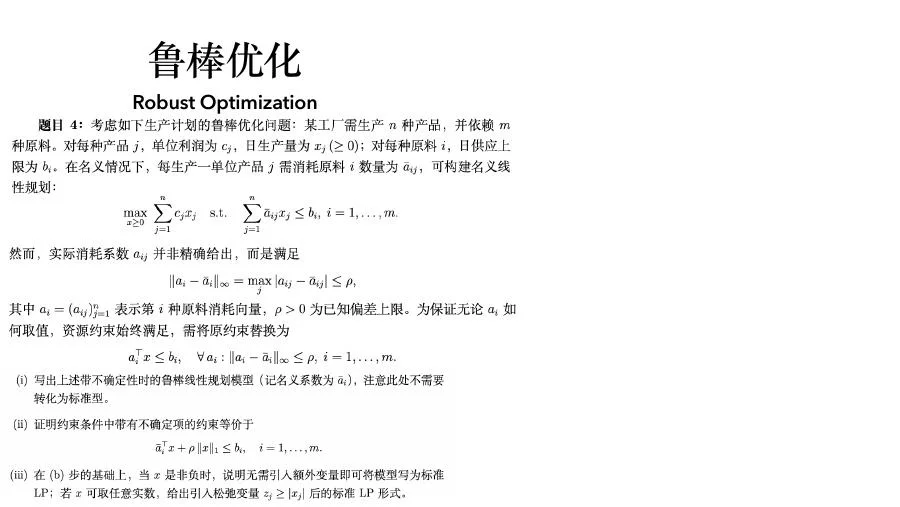
Suppose a linear constraint must hold for every uncertain coefficient:

The robust counterpart protects feasibility over the chosen uncertainty set. Wider sets increase protection but can make the plan conservative. The uncertainty set must be calibrated from data, engineering bounds, or clearly stated scenarios.

Robustness is not the same as adding an arbitrary safety factor. It specifies exactly which values vary together and which constraints must survive.

What “for every value” really demands

Start with a constraint you already know: product I uses two kilograms of material per unit, product II uses one, and the factory has eleven kilograms. The ordinary rule is. Suppose those usage numbers were estimates. Product I might use between 2.0 and 2.2 kilograms per unit; product II between 1.0 and 1.1. If we require feasibility for every combination of these intervals and, the most demanding combination uses the upper ends of both intervals. The robust rule becomes. It is still a linear inequality. The protection did not come from saying “add ten percent”; it came from a declared uncertainty set and a worst-case calculation.

Try the nominal profit maximum. Its estimated material use waskg. Under the upper-end usage coefficients, it may needkg. It therefore fails the robust rule. Try the balanced continuous plan. Its upper-end material use iskg, exactly the limit. This is a different uncertainty story from the earlier one-kilogram supplier shortfall. There, the coefficients stayed at 2 and 1 but capacity fell from eleven to ten. Both stories happen to favor the same continuous balanced plan with these numbers, yet their worst-case mechanisms are distinct. If both usage inflation and supplier shortage can occur together, the balanced plan may no longer be protected: upper-end usage needs eleven kilograms but the short supplier delivers ten. Never claim robustness against a combined event you did not put in the uncertainty set.

The phrase “every combination” is powerful and potentially conservative. Are both recipes likely to use their worst material quantity on the same day? If their extra usage comes from a common quality problem, perhaps yes. If their deviations are independent and bounded through laboratory measurements, a full box of joint extremes may protect against a very rare combination. A budgeted uncertainty set can limit how many coefficients move to their extremes at once. An ellipsoidal set can express a joint Euclidean deviation region. We choose a geometry because it represents what we know about simultaneous deviations; we do not choose it merely because a solver has a convenient command for it.

Here is the ellipsoid idea in one algebra step. Let the uncertain coefficient vector be, whereis the nominal vector,sets the scale and directions of coefficient errors, and. Then the worst possible value ofisby the Cauchy–Schwarz bound, with equality in the adverse direction when allowed. The robust constraint can be written. The norm term is why a second-order cone form can appear. Ifis a diagonal matrix of independent scales, the term measures the combined exposure of the chosen production mix to coefficient uncertainty. The more of an uncertain product we make, the larger the protective term. We should still explain whatandmean in kilograms, not only show a norm.

What is the price of robustness? Compare each robust plan’s nominal objective with the nominal optimum under identical profit coefficients. In the supplier-shortfall example, protecting against one kilogram costs 20,000 yuan of nominal profit in the continuous model. Under the interval-coefficient example, the same numerical drop happens, but it protects against a different event. We should also compare worst-case feasibility and actual observed violation rate if we have held-out days. An uncertainty set calibrated too narrowly may give a low price and many real failures. A set calibrated far wider than evidence or engineering bounds may waste profit for protection against impossible combinations. Price alone cannot evaluate calibration.

You might ask why we did not simply use a chance constraint, requiring the material rule to hold with probability at least 95%. That is a different promise. It permits up to a stated violation probability under a credible distribution, whereas robust feasibility over a set permits none inside the set and says nothing about events outside it. A 95% guarantee also needs careful interpretation: an estimated probability can be wrong when the sample is small or the distribution shifts. The factory owner may accept occasional short production but not a hard contract violation. We should match the mathematical promise to the real consequences.

Finally, distinguish uncertain decisions from uncertain measurements. The number of product unitsis chosen; material coefficients and delivered stock are external inputs. We may optimize the production mix to manage uncertain material use, but we should not write “the solver chooses the uncertainty” unless we are modeling an adversary in a well-defined minimax sense. The robust inner maximization is a test of a candidate plan against allowed bad data, not a claim that a malicious supplier controls every kilogram.

Stochastic and scenario models

When probabilities are meaningful, minimize expected cost plus a risk measure:

For two-stage decisions,is chosen before the scenario is known and recourseis chosen afterward. Scenario probabilities must not leak future knowledge into the first-stage decision.

Decide when the factory can react

Imagine the supplier either delivers all eleven kilograms of material tomorrow, with probability 0.8, or delivers only ten, with probability 0.2. These are illustrative probabilities chosen to teach the calculation; a real factory would estimate them from delivery history and ask whether seasons or suppliers change the rates. On the day before delivery, the factory might commit to customer orders and reserve machine time. On the morning of delivery, it might purchase emergency material or change the product mix. The model must say which of these actions occurs before and which after the uncertainty is observed.

The nominal profit-maximizing continuous planearns 620,000 yuan if all eleven kilograms arrive. On a ten-kilogram morning it needs one missing kilogram. Suppose a guaranteed emergency supplier will sell that kilogram for 30,000 yuan, with immediate delivery and no other hidden delay. Then the same production plan earns 590,000 yuan net on that short day. Expected net profit across the two states isyuan. The protected balanced planearns 600,000 yuan whether ten or eleven kilograms arrive under the nominal usage coefficients. With this reliable emergency option and these probabilities, a fixedcommitment plus recourse has a higher expected modeled net profit by 14,000 yuan.

That conclusion depends on the emergency option being real. If the backup supplier has no spare stock, arrives after the production deadline, or charges a large setup fee, the ten-kilogram day cannot be repaired as assumed. The nominal plan might then breach a customer contract; the associated penalty and lost trust may dwarf a 20,000-yuan profit difference. A stochastic model does not automatically make risky plans safe. It makes the decision timing and recovery action explicit, so we can test whether the recovery exists.

What emergency price flips the expected-profit comparison? Letbe the net cost, in yuan, of correcting a one-kilogram shortage. The nominal plan’s expected profit is, while the protected plan earns. They tie when, soyuan. If emergency correction costs more than that under this toy probability, the protected plan has higher expected net profit. If the shortfall probability changes, the threshold changes inversely. For example, a 0.1 shortfall probability would double the break-even emergency cost. The point is not to recommend an expensive kilogram purchase; it is to show exactly which assumption controls the preference between here-and-now protection and recourse.

Now add the factory’s soft balance preference. The nominal plan produces one more I than II; the protected plan is balanced. Even if the nominal-with-recourse policy wins by 14,000 yuan in expected profit, the manager might prefer the balanced plan for catalog or customer reasons. That preference is separate from delivery uncertainty. We can present a table with expected profit, worst short-day net profit, material feasibility, and imbalance, then let the manager choose with the consequences visible. One scalar “best score” could hide the trade-off again, undoing the work we did at the start of the lesson.

There is a subtler two-stage possibility: commit only to a minimum delivery level now and choose the extra production after material arrives. That requires a set of customer contracts with flexible quantities and machine capacity that remains available. The first-stage contract may be more conservative than the eleven-kilogram optimum, while the morning recourse uses additional stock if present. We would need variables for committed units and scenario-specific additional units, plus constraints that prevent retracting commitments after seeing the short scenario. If we instead let all production quantities depend on the scenario, we have effectively assumed perfect information before committing. It might describe a factory that really waits until delivery to take orders, but it does not describe one that promised products the night before.

The city energy example has the same timing. Day-ahead gas and wind arrangements are first-stage. Emergency gas or shortage after weather is revealed is recourse. Stating the order of events is often more important than the name of the stochastic solver. A student who can point to the clock in the story can usually avoid the most damaging form of future-information leakage.

Communicate the decision

Show at least three points: a low-cost extreme, a balanced compromise, and a high-protection extreme. For each, report objective values and binding constraints. Then stress-test all candidates under the same scenarios.

The recommended plan should come with a policy: which parameter is monitored, what threshold triggers reconsideration, and which alternative becomes preferable. A trade-off plot plus a trigger rule is more actionable than one “optimal” number.

Suppose we have to speak to the factory manager today, not after another week of mathematics. I would put three plans on one page. The continuous profit-only planearns 620,000 yuan with eleven kilograms of material, fills ten machine-hours, and makes one more I than II. It is impossible if material arrives one kilogram short and no backup exists. The continuous balanced planearns 600,000 yuan, uses ten kilograms, fills machine time, and remains feasible under that one-kilogram shortfall when recipe coefficients stay nominal. The integer planearns 560,000 yuan, uses eight kilograms, fills machine time, and meets the no-excess-I rule. The fractional plan belongs on the page only if divisible production is actually permitted; otherwise it is a benchmark, not a schedule.

How should the manager read that page? If contracts require whole units and prohibit excess I, the integer plan is the immediately executable option among these, and we must compare it with other integer plans before declaring optimality. With the tiny slide limits, enumeration shows it is indeed the highest-profit integer plan satisfying: if, at most five II give profit 50; if, at most four II give 48; if, four II give 56; if, three II give 54;withviolates the ten-hour machine limit. All profits here use the slide’s ten-thousand-yuan scale. This hand check ties the integer recommendation to the actual feasible grid rather than to rounded fractions.

If production can be divided, the continuous balanced plan is more profitable than the integer one and protects against the declared stock loss. If the manager allows imbalance and has guaranteed emergency material, the profit-only plan may win in expected net profit under some emergency price and shortage frequency. The policy could say: “Use the balanced plan if the confirmed material is ten kilograms or if no emergency supplier is available; consider the nominal plan only when the eleven-kilogram supply and imbalance permission are both confirmed.” A monitoring trigger is not an afterthought. It tells the factory which observation changes the choice.

The city energy planner needs the same kind of page. List normal-day dollars, direct operational emissions, calm-day shortage, and whether emergency purchase is available. The recommendation should identify a reliability ceiling or a shortage penalty that has been approved by the decision maker. “Choose 70/30 under a zero-calm-shortage rule” is defensible in the toy model. “Choose 70/30 because our algorithm likes it” is not. A policy statement lets another analyst update the choice when weather forecasts, emergency gas prices, or legal standards change.

There is also a communication test: can a reader reproduce one trade-off from the page without opening the code? The manager should see that moving from the profit-only to balanced factory plan costs 20,000 yuan nominally and frees one kilogram. The city planner should see that moving from 70/30 to 50/50 saves 800 normal-day dollars, lowers direct emissions by eight tonnes, and increases calm shortage by twenty MWh without recourse. If those arithmetic comparisons are absent, the frontier plot becomes a pretty curve detached from the actual decision.

Before publishing either recommendation, I would ask a teammate to play the role of the skeptical decision maker. They should not need to know the name of the solver. For the factory they might ask, “Are the quantities whole, and what if the truck brings only seven kilograms?” We can answer: the continuousrecommendation is not a whole-unit schedule, the whole-unit balanced alternativeuses eight kilograms, and the 560,000-yuan target cannot be met under the stated continuous model when stock falls below eight. That last answer may be uncomfortable, but it is exactly the kind of warning the manager needs before committing to customers. If emergency material is available, we should give its actual cost and arrival time rather than answering with an abstract “recourse variable.”

For the city they might ask, “Does your clean option keep the lights on at a hospital?” Our toy 50/50 and 30/70 choices have calm-day shortages of 20 and 40 MWh without backup, so the answer is no under the zero-shortage interpretation. We can either restrict the feasible set to zero shortage, model an independently reliable backup, or explain that some noncritical demand may be curtailed while critical demand remains supplied. The table’s single total-shortage number cannot tell us which loads fail. A public recommendation would need a priority model and network feasibility checks. Teaching a Pareto frontier should not make us forget who bears the adverse outcome.

These questions reveal why the final output should show assumptions beside the figures, not in an appendix nobody reads. The factory comparison assumes constant unit profits, continuous production for two of the plans, and either a specified emergency option or none. The energy comparison assumes normal-day wind availability 70 MWh, calm availability 30, fixed gas commitments, direct operational emissions only, and a toy shortage penalty when expected dollars are calculated. The result changes when an assumption changes; the page should make that dependence easy to see. A strong recommendation is one that can be revised honestly, not one that sounds permanent.

If a later observation contradicts the model, start with the assumption that observation tests. A short factory delivery tests the material-capacity promise; a calm-day electricity deficit tests wind availability and backup. Updating the relevant input and re-solving is more informative than defending the old optimum. That is how a modeling lesson becomes a decision process.

Pareto, robust, and scenario methods each answer a slightly different question. We will give a manager a small set of options and practice saying what each method assumes before recommending one.

Choose under competing objectives

Suppose a city must choose an electricity portfolio. Technologyhas annual cost, expected emissions, reliable capacity, and uncertain outputin scenario. The decisionis installed capacity. Cost, emissions, and reliability cannot be collapsed until their units and trade-offs are understood.

Let us make the abstraction feel like a conversation. A city planner asks, “Should we lean on cheap clean power or retain a larger amount of dependable fuel-based supply?” The question is not answered by shouting “renewables” or “reliability.” It asks for a comparison of money, emissions, and unmet demand when weather is unfavorable. We need a time horizon and a system boundary before we can compare them. For a one-day teaching example, we will ignore construction cost and use energy quantities. For an actual installation decision, construction, lifetime, storage, network constraints, and dispatch would all return.

A one-day example before the general model

Suppose the city needs 100 MWh tomorrow. It can prearrange gas-backed energy at 90 dollars per MWh, emitting 0.4 tonnes of carbon dioxide per MWh, or wind-backed energy at 50 dollars per MWh with no direct operational emissions in this toy boundary. In normal weather, up to 70 MWh of wind is available. In a calm scenario, only 30 MWh is available. For now assume the city cannot buy additional gas after making the day-ahead choice. Letandbe the gas and wind energy quantities arranged, with,, and.

We could select. Normal-day cost isdollars; operational emissions aretonnes. The calm-day wind supply of 30 MWh still matches what we planned, so modeled shortage is zero. We could instead select. Normal-day cost drops todollars, and emissions to 20 tonnes, but calm-day wind contributes only 30 MWh; with 50 MWh of gas arranged, total supply is 80 and shortage is 20 MWh. An aggressive choicecostsdollars and emits 12 tonnes on the normal schedule, but calm-day shortage reaches 40 MWh. The cheap clean choices are not “bad” by definition; they trade off against a reliability outcome the city must value.

Put those outcomes in one table, all with the same system boundary:

Day-ahead choice	Normal-day cost ($)	Normal-day operational emissions (t)	Calm-day shortage (MWh)
70 gas, 30 wind	7,800	28	0
50 gas, 50 wind	7,000	20	20
30 gas, 70 wind	6,200	12	40

Read the table aloud. Every additional 20 MWh of planned wind saves 800 dollars and eight tonnes of modeled emissions in normal weather, but adds twenty MWh of shortage in the calm scenario. This is the Pareto pattern. None of the three rows dominates another when cost, emissions, and calm shortage all matter: the better price and emissions arrive with worse shortage. A fourth row with 100 MWh of gas would cost 9000 dollars, emit 40 tonnes, and have zero calm shortage; the 70/30 row is no worse in shortage and better in the other two measures, so it dominates the all-gas row under the declared assumptions. This is why we remove dominated candidates before asking stakeholders to choose: a dominated row has no compensating advantage in the outcomes we agreed to evaluate.

The example is intentionally narrow. Gas also has uncertain availability and price in real markets; wind may create lifecycle emissions and grid-balancing costs; the city may store energy or trade with neighboring networks. We have defined direct operating emissions rather than lifecycle emissions, and normal-day contracted energy cost rather than total ownership cost. If a policymaker asks a broader question, we expand the model rather than stretch our toy table beyond its meaning. A course tutorial should make this boundary visible at the same moment it teaches the mathematics.

Build the feasible set first

Write physical and policy constraints before preferences:

Hereis allowed shortage or recourse. A plan outside this set is not a “less preferred” plan; it is infeasible. Separating feasibility from preference prevents a weighted objective from silently buying violations that should be impossible.

In the toy table,is a normal-day energy balance, not a promise of calm-day supply. If the city has a legal requirement of zero shortage even in calm weather and no recourse, it must impose. With, this reduces to. Under that hard reliability rule, the 50/50 and 30/70 rows are not “less preferred”; they are disallowed. The cheapest normal-day plan inside the rule is the 70/30 row. If a small calm shortage is acceptable, perhaps the policy states “no more than 20 MWh,” and the 50/50 row becomes legal. A precise reliability threshold turns a broad value debate into a constraint that a reader can check.

This is the role of the epsilon-constraint idea in ordinary language. We can minimize normal-day cost subject to a calm-shortage ceiling oforMWh. Each ceiling gives us another feasible decision and another point on the trade-off curve. We can display the ceiling itself beside the result. The city then chooses a visible tolerance rather than trusting an unexplained weight that mixes dollars, tonnes, and megawatt-hours. There may still be politics in the threshold, but it is politics the report has made explicit.

Construct a Pareto frontier

First minimize cost alone and emissions alone. These anchor solutions reveal scale and conflict. Next use the epsilon-constraint method:

Sweepacross a meaningful range. Remove dominated points: solution A dominates B if A is no worse in every objective and strictly better in at least one. A weighted sum can miss non-convex parts of a frontier, while epsilon constraints can expose them.

With this simple two-source toy, normal-day cost and emissions both fall asincreases, while calm shortage rises after. For planned wind below 30, increasingimproves cost and emissions without creating calm shortage, so those lower-wind rows are dominated. Fromthrough, further wind is a genuine trade-off. The frontier begins at the zero-shortage row; it does not begin at all-gas merely because all-gas sounds safe. Computing single-objective anchors and removing dominated points can discard an option that a naive presentation would treat as a serious “high reliability” extreme.

In a larger energy system, cost and emissions need not move together. A low-cost fossil source might raise emissions, a low-emission technology might cost more, and geographically diversified supply might improve reliability without changing the total renewable share. The frontier may be a surface rather than a simple curve. We should not force it into a one-dimensional slogan. The toy shows the reasoning mechanism; the full model must use actual technology, demand, and network data.

Select a compromise only after showing the frontier. A knee point is where a small further improvement in one objective requires a large sacrifice in another, but “knee” must be supported by a curvature rule or stakeholder reasoning rather than visual preference alone.

Model decisions before and after uncertainty

Installed capacity is chosen before scenariois observed; dispatch and shortage are chosen afterward. This produces a two-stage stochastic program:

whereis the optimal recourse cost in scenario. A perfect-information benchmark allowsto depend onand is unrealistically optimistic. The difference between perfect-information and here-and-now objectives measures the value of knowing the future.

Our toy assumed no after-weather action. What if the city can arrange emergency gas after learning the wind output? Then we need two times in the model. A day-ahead commitment is made before weather is known; emergency purchase is made later. This recourse could make a 50/50 plan viable on calm days, but only if there is enough physical gas and the premium price is included. If emergency gas costs 150 dollars per MWh, the 50/50 plan needs 20 emergency MWh in calm weather, adding 3000 dollars on that day. The 30/70 plan needs 40, adding 6000. The expected premium depends on the likelihood of calm weather, which we must estimate or openly use as an assumption. We cannot charge the day-ahead plan the cheap gas price for emergency supply after the event.

The perfect-information comparison would let us choose a different day-ahead portfolio after seeing whether the day will be calm. It can give a lower cost than any genuine day-ahead policy because it is allowed to know what the planner did not know. We may calculate it as a benchmark for the value of information, but we cannot present it as an implementable schedule. A table may contain beautiful scenario-specific decisions that are impossible to make at the time the real decision is due. Label every variable by its decision time. Ifis here-and-now, it must have one value across scenarios; only recoursemay differ after scenariois observed.

Include risk, not only expectation

Two portfolios can have the same expected cost but very different tails. Conditional Value at Risk at levelsummarizes the mean loss in the worstfraction of cases. For loss,

$$
\operatorname{CVaR}\alpha(Z)=
\min_\eta\left[\eta+\frac{1}{1-\alpha}\mathbb E(Z-\eta)+\right].
$$

Explainas a loss threshold andas excess loss. Increasing the CVaR weight purchases protection at an expected-cost premium. Plot both quantities.

We can quantify why expectation may feel too calm. Suppose a calm day occurs with probability 0.2 and we assign an illustrative shortage loss of 300 dollars per unserved MWh. With no emergency purchase, the 70/30 row has zero shortage penalty. The 50/50 row incursdollars on a calm day and zero otherwise, so expected shortage penalty isdollars. The 30/70 row incursdollars on a calm day, with expected penalty 2400 dollars. Adding normal-day energy cost gives illustrative expected totals of 7800, 8200, and 8600 dollars. Under this probability and penalty, the reliable 70/30 plan is also cheapest in expected modeled cost. Under a much smaller shortage penalty or a rarer calm day, the ranking can change. That sensitivity is a result, not an inconvenience.

At CVaR levelin this two-scenario example, the worst 20% of days are exactly the calm days if they carry the largest shortage losses. The CVaR of shortage penalty is therefore 0, 6000, and 12000 dollars for the three rows. If calm probability were 0.05 rather than 0.2, the worst 20% tail would include some normal days too, so the calculation would differ. CVaR is not a decorative risk word. It is a specific average of the adverse tail under an assumed distribution. Report both the distribution and the cost measure before quoting it.

There are at least three honest ways to tell the city what to do. A risk-neutral planner might minimize expected dollars including shortages. A planner with a zero-shortage obligation might choose a robust constraint. A planner able to tolerate rare interruptions but not extreme ones might minimize expected cost plus a tail-risk measure. None of these is “the algorithm that handles uncertainty” in the abstract. Each expresses a different institutional promise. That promise belongs in the recommendation sentence.

The probability itself may be uncertain

Our arithmetic used a calm-day probability of 0.2. Where did that number come from? In a real energy study we could count historical days with wind output below the relevant threshold, stratify by season, compare weather records with the coming day’s forecast, and check whether the next year looks like the sample. If we observed two calm days in only ten recorded days, the empirical fraction is 0.2, but ten days are far too few to treat 0.2 as an exact natural constant. Even an excellent optimization algorithm cannot recover a reliable tail frequency from a tiny or biased sample.

The city toy lets us calculate a switching probability. After, each additional planned wind MWh saves 40 normal-day dollars because wind costs 50 instead of gas 90. It also creates one additional MWh of shortage on a calm day when no recourse exists. At a 300-dollar loss per unserved MWh and calm probability, the expected shortage cost per extra wind MWh is. So expected modeled cost decreases with more wind when, increases when, and is flat when. At, the aggressive 30/70 choice has normal cost 6200 plus expected shortage loss, totaling 7400 dollars, below the reliable 70/30 choice’s 7800. At, it totals 8600 and loses. The preferred plan switches between those probability assumptions. That is a much more informative statement than “the solution is sensitive.”

The shortage price is equally uncertain. If a calm shortage affects only a deferrable industrial load, 300 dollars per MWh might be an overestimate. If it interrupts a critical hospital supply, money may be the wrong language entirely; a zero-shortage constraint or separate emergency backup rule may be required. If emissions are priced by an approved policy, an extra wind MWh also saves 0.4 tonnes of direct emissions, changing the monetary threshold. We must keep consequence, probability, and preference separate in the report. A sensitivity grid overand the shortage loss can show where each plan wins, but its axes need clear units and a statement that the toy excludes network and storage effects.

At CVaR level 0.8 with exactly 20% calm probability, the worst tail contains the calm losses. Yet if we admit probability uncertainty, a tail estimate can move dramatically. A single extra calm day in a short dataset may change both the estimated frequency and the shortage-loss tail. Instead of printing a CVaR to six decimals, report the data window, loss definition, and plausible interval across scenarios or bootstrap samples. Risk measures are summary statistics of an assumed distribution; their precision should not exceed the credibility of that distribution.

How might a planner respond whenis not stable? One option is to evaluate the three portfolio rows over a range such asand show regret relative to the best plan at each. Another is to choose a policy that adjusts day-ahead energy commitments after a reliable forecast arrives, with the forecast time stated explicitly. A third is to install emergency capacity whose value grows on calm days. Each response changes the decision timing or feasible set. None is achieved by silently replacing 0.2 with a favorite number. The graph of switching regions should lead to an operational monitoring rule: what forecast or supply indicator would trigger a different commitment, and how late can we change it?

Strategic uncertainty and game theory

Some uncertainty comes from another decision maker rather than nature. If two firms choose prices, or defenders allocate resources against an adaptive attacker, scenarios with fixed probabilities may be inappropriate. A payoff matrix can reveal dominant strategies, best responses, and Nash equilibria. In a zero-sum finite game, mixed strategies solve a linear program. State whose incentives are modeled; “opponent chooses the worst scenario” is a robust model, not automatically a behavioral theory.

When tomorrow’s “uncertainty” is another person

To see the difference, imagine two small cafés on the same street choosing a high or low lunch price. Use fictional payoff numbers measured in thousands of yuan of daily profit. If both choose high, each earns four. If A chooses low while B chooses high, A earns six and B one because customers switch toward A. If A chooses high while B chooses low, the payoffs reverse. If both choose low, each earns two. The matrix is a model of incentives, not a weather forecast. We are not saying a café literally has a 20% chance of low-price weather; the other owner chooses a response.

Ask café A what it prefers if B chooses high. A gets six from low rather than four from high. If B chooses low, A gets two from low rather than one from high. Low is therefore A’s best response in either case. By symmetry low is B’s best response too. The pair low/low is a Nash equilibrium in this toy matrix: neither café improves its own payoff by changing alone. Both would earn more at high/high, but either café has an incentive to undercut that arrangement. This is why modeling strategic uncertainty differs from merely enumerating fixed scenarios with assigned probabilities. The probability of B’s action may itself depend on A’s action, past behavior, and incentives.

What would a robust planner do here? It might choose A’s price to maximize A’s worst payoff over B’s possible choices. In this particular matrix, A’s worst payoff from high is one, while from low it is two, so robust maximin also selects low. It happens to match the equilibrium here, but it arrived by a different argument. Maximin treats B as an adverse scenario set; equilibrium studies both actors’ best responses. In another matrix those choices can disagree. Do not call a robust worst-case calculation a Nash equilibrium unless both players’ incentives and response rules were actually analyzed.

The course mentions games alongside uncertainty for a reason. Some “unknown” inputs are physical randomness, some are measurement uncertainty, and some are choices made by other agents. Electricity wind output is mostly an external physical event in our toy example. A rival’s price or an adaptive defender’s action is strategic. A supply delivery can mix both if suppliers respond to our purchase contract. Name the source of uncertainty before choosing a mathematical treatment. Otherwise a precise scenario probability may conceal a mechanism that changes when we change our own policy.

Practice

Create five candidate portfolios and calculate cost, emissions, and worst-scenario shortage. Identify dominated alternatives. Then formulate the continuous portfolio model, generate an epsilon-constraint frontier, and select three representative solutions. For each, report expected cost, CVaR, maximum shortage, active constraints, and the parameter range over which it remains preferable.

Course example: three goals in production

The base two-product data: raw-material use, equipment time, profit, and available capacity.

The three soft goals: balance the two products, use equipment fully, and reach at least 560,000 yuan profit.

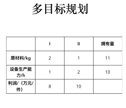
	Product I	Product II	Available
material (kg)	2	1	11
machine time (h)	1	2	10
profit (10,000 yuan)	8	10	—

The feasible set is,,. The course adds three aspirations: keep product I from exceeding II, use the machine fully, and earn at least 560,000 yuan. Turning all three into hard constraints can make the model infeasible, so goal programming introduces deviations:

Begin with a plan a manager can understand

The units are small, so we can reason on paper.is how many units of product I we make;is how many units of product II. Each I consumes two kilograms of material and one machine-hour; each II consumes one kilogram and two machine-hours. We have eleven kilograms of material and ten machine-hours. The profit coefficients are in ten-thousand-yuan units, socorresponds to 560,000 yuan. If we forget that scale and report “profit 56 yuan,” every later comparison would be nonsense.

Try a plan before optimizing: make three of each. Material use iskg, and machine use ishours. Profit is, or 540,000 yuan. This plan is legal and balanced, but it misses the 560,000-yuan aspiration and leaves one machine-hour idle. It is a useful baseline precisely because we can calculate every shortfall by hand. A feasible baseline is not an embarrassment; it tells us what each improvement costs.

Where is the profit-only optimum? The material and machine boundary lines intersect atand. Solving gives. Check: materialkg, machinehours, profit, or 620,000 yuan. The other axis corners arewith profit 44 andwith profit 50 in the same units. Thusis the continuous profit maximum. It fully uses both resources, but produces one more unit of I than II. The manager’s balance wish is the one aspiration it violates.

Is balance a legal prohibition or a preference? Ask the manager. If “product I may never exceed II” is a hard contractual rule, addand search the restricted feasible region. If the rule is “we would prefer a balanced catalog but will accept some imbalance for a good profit,” it is a soft goal. Treating a preference as hard can exclude economically attractive plans; treating a safety or contractual rule as a penalty can allow illegal plans if the profit incentive is large enough. Before writing deviation variables, determine which kind of sentence the manager has actually said.

For a hard no-excess-I rule, a particularly informative plan lies at. Machine use ishours; material use iskg; profit is, or 600,000 yuan. It is balanced, fills the equipment schedule, and exceeds the 560,000-yuan target. Compared with, it sacrifices 20,000 yuan of profit while saving one kilogram of material and removing the imbalance. That 20,000 yuan is the price of the specific fairness restriction under these continuous data, not a universal exchange rate between fairness and money.

You may notice thatunits of each product is fractional. If units are indivisible, this continuous plan is an upper benchmark rather than an immediately executable schedule. Try integer plans:is balanced but earns 540,000 yuan, whileis balanced, useskg of material andhours, and earns, exactly 560,000 yuan. Under the hard balance and the declared target,is an executable candidate. We would still enumerate or solve the integer model before declaring it the best legal integer plan. This is why “goal programming” does not eliminate the need to define domains.

Now return to soft wishes. For product balance, the expressionis positive when I exceeds II and negative when II exceeds I. Introduce nonnegative deviationsand write. If, one consistent choice is. If, the corresponding under-balance deviation is. The course wish penalizes excess I, not necessarily excess II, so onlybelongs in that particular penalty. Penalizing both directions would impose a different notion of balance. We should say which one we mean.

For machine use,. Since machine capacity is a hard rule,remains in the model. We then interpretas unused hours, not as permission to violate capacity. At,. Atand, it is zero. If we dropped the hard capacity inequality and only penalized, a high-profit plan might buy a machine-hour violation through the objective. That would be a modeling error if the machine physically cannot operate for eleven hours.

For profit,. A plan earning 54 hasin ten-thousand-yuan units, meaning a 20,000-yuan shortfall. A plan earning 62 has, meaning it exceeds the aspiration by 60,000 yuan. If the manager cares only about not falling short, penalizeand do not penalize the positive surplus. Goal equations describe deviations; the objective decides which deviations are regrettable.

Penalizefor excess I,for unused equipment, andfor profit shortfall. Normalize units. With priorities, minimize profit shortfall first, fix it, then improve utilization and balance. This is more transparent than one unexplained weighted sum.

Let material arrive before choosing production

The production numbers let us show why decision timing matters using one family of equations. Suppose the factory does not promise exact quantities the night before. It waits for the material truck, sees whether the delivered quantity is 9, 10, or 11 kilograms, and then chooses production. Keep machine time at ten hours and maximize profit under the observed material amount. In the range where both material and machine limits bind, solveand. The answer isand. Atit makesof I andof II, earning 58 units of 10,000 yuan. Atit makesof each and earns 60. Atit makesand earns 62. Each one-kilogram increase in this local range raises the best continuous profit by two units of the slide scale, or 20,000 yuan.

This small sequence teaches several things at once. Under nine kilograms the model shifts toward product II, which uses less material per profit opportunity in this constrained regime. At ten kilograms the mix is balanced. At eleven it makes one extra unit of I, violating the manager’s soft balance wish. The material supply does not merely lower a final number; it changes the product mix and the manager’s preference trade-off. If the balance wish becomes a hard rule, theprofit-only point is excluded even though material is plentiful. That is another clean separation between uncertain data and declared values.

Suppose eleven kilograms arrive with probability 0.8 and ten kilograms with probability 0.2. If the factory can genuinely wait until delivery before choosing quantities and customers accept that flexibility, the adaptive policy earnsyuan in expected modeled gross profit. Compare that with the fixedplan plus the earlier emergency purchase at 30,000 yuan, which earned expected net profit 614,000, and the fixed protected plan, which earned 600,000. The adaptive policy is better under this toy setup because it changes mix on the short day without emergency cost. But it may not be available if the factory promised four I and three II in advance. The 616,000 figure is not a free improvement delivered by “stochastic optimization”; it is the value of a particular operational flexibility.

The formula has a range of validity. It comes from intersecting both active boundaries. Iffalls below five kilograms, the machine may no longer be fully used at the optimum because even five units of product II require five kilograms. Ifbecomes very large, material may stop binding. Do not extrapolate the local 20,000-yuan-per-kilogram slope to all possible material supplies. A sensitivity result is honest only when it states which active constraints support it and where those constraints might change.

If units are whole, the fractional adaptive mixes are again benchmarks. We would solve or enumerate an integer plan for each delivered amount and compute its scenario profits separately. A student might be tempted to roundtoon a nine-kilogram day. That rounded plan needskilograms and is infeasible. Rounding is not a recovery policy. Re-solving the legal grid is.

The production example produced a candidate decision. Now we ask whether it remains reasonable when objectives or inputs move, rather than presenting one weighted score as if it ended the discussion.

Pareto and robustness reasoning

A plan dominates another if it is no worse in every objective and better in one. Generate a frontier by maximizing profit while limiting imbalance and requiring utilization across a range of thresholds. Present knee points and the marginal price of fairness.

If material availability is,, a simple robust counterpart uses. More general budgeted sets restrict how many coefficients become adverse together. Calibrate the robustness budget from data. Then compare nominal and robust plans by expected profit, worst loss, violation frequency, and price of robustness.

Compare regret, not just raw expected dollars

Return to the city table with no emergency supply, a 300-dollar shortage loss per MWh, and calm probability. At, modeled expected totals are 7800 dollars for 70/30, 7600 for 50/50, and 7400 for 30/70. The aggressive plan is cheapest under that assumption. At, totals are 7800, 8200, and 8600; the reliable plan is cheapest. We can express regret as a plan’s modeled cost minus the cheapest cost under the same:

Plan	Regret at($)	Regret at($)
70 gas, 30 wind	400	0
50 gas, 50 wind	200	400
30 gas, 70 wind	0	800

Read this as a consequence table, not a ranking invented by the model. If the city’s best estimate is, the aggressive row has no modeled regret. If the city fears the estimate may actually be, its regret is 800 dollars. The reliable and middle rows have a largest regret of 400 dollars over just these two tested probability values. A minimax-regret rule across the two values would tie them; an additional criterion such as emissions, more probability values, or a legal shortage ceiling would break the tie. We should not convert a two-point regret table into a universal safety claim. It is a transparent view of what the mistaken probability assumption would cost under the toy loss model.

This also shows why a single “balanced compromise” cannot be chosen by appearance alone. The 50/50 row looks visually central, yet it is never the lowest expected-cost row at either tested probability. It may still be preferable to stakeholders because it offers a different emissions and shortage combination or because it limits the largest regret. State the reason. A manager should be able to tell whether a recommendation came from an approved reliability constraint, a tail-loss criterion, a regret criterion, or an informal midpoint. If we cannot tell, the mathematics has not finished the communication job.

The factory has a similar regret question. Choosing a fixed robust mix leaves nominal profit on the table on full-supply days; choosing a nominal mix without real recourse risks infeasibility on short days. A table can show profit loss relative to the best legal plan after supply is known, but it must not then pretend the best-after-supply plan was available before supply was known. Regret is a comparison device; timing still governs what can actually be chosen.

The one-kilogram shortfall changes the preferred plan

The profit-only planconsumes all eleven kilograms of material. If the supplier arrives one kilogram short, only ten kilograms are available; the old plan is impossible before production even begins. A robust plan under a declared one-kilogram shortfall must satisfyas well as the ten-hour machine limit. Their intersection is, exactly the balanced continuous plan we found. Its profit is 600,000 yuan, 20,000 below the nominal profit maximum, and it remains feasible with ten kilograms of material. The numerical coincidence is useful for teaching but not a general theorem: in other data, the robust plan and the fairness-constrained plan can be different.

What should we call the 20,000-yuan difference? For this one worst-case material scenario, it is the nominal price of protection against a one-kilogram supply loss in the continuous model. But it does not tell us whether the purchase is worthwhile. If that shortfall happens once in a hundred days and unused material can be purchased urgently, a policy with recourse might do better. If it happens frequently and missing production causes contract penalties, worst-case feasibility may be valuable. We need scenario frequencies or credible bounds, plus costs of late procurement, before choosing robust protection by habit.

Suppose the factory can order emergency material after seeing the morning delivery, but at a high premium. The morning production decision might include a first-stage schedule, while emergency procurement is a second-stage recourse action. A robust “produce less every day” plan and a stochastic “produce nominally, buy material on rare short days” plan answer different questions. The latter requires credible probabilities and a clearly available emergency supplier. If no supplier exists at the deadline, emergency recourse is fictional, no matter how elegant the stochastic program looks.

This returns us to the chapter’s two separate difficulties. The manager’s balance preference can lower profit even with perfectly known material; the material shortfall can lower profit even if the manager cares only about profit. In our tiny numbers both pressures moved the continuous answer toof each product, but we should not combine them into a single vague word like “risk.” Tell the decision maker what changed because of value judgment and what changed because of an uncertain input. A transparent trade-off is easier to revisit when priorities or supply reliability change.

Which aspiration fails first when supply shrinks?

We can now return to the manager’s target of at least 560,000 yuan and ask a practical question: how low can material supply fall before the target becomes impossible, assuming continuous production and ten machine-hours? The local solution from the intersection of the material and machine limits earnsunits of 10,000 yuan when material supply iskilograms in the relevant range. To reach the target 56, we need, or. At exactly eight kilograms, the intersection gives, profit 56, zero excess I, and full machine use. This is also an integer plan. It meets all three aspirations under that capacity, but has no profit cushion against another supply loss.

At seven kilograms, the continuous profit maximum from these two active boundaries isand profit 54, or 540,000 yuan. If the manager turns “at least 560,000” into a hard rule, the model is infeasible at seven kilograms under the stated ingredients and ten machine-hours. If it is a soft aspiration, the model can still select a legal plan and report a shortfall of at least 20,000 yuan. The difference between “cannot operate” and “operates below target” comes from whether the target is hard or soft. This is exactly the kind of distinction goal programming was designed to make visible.

Do not stop at the algebraic threshold. Ask whether the profit coefficients remain valid if only a few units are produced. Maybe the factory pays a fixed setup cost for each recipe, in which case the 540,000-yuan gross figure is not net profit. Maybe customers order only whole units, in which case the fractional seven-kilogram point is not executable. Maybe material can be substituted or bought at short notice. These are reasons to revise the model and re-evaluate the threshold, not reasons to suppress the threshold altogether. The simple calculation still tells us where additional data or recourse could be most valuable.

This threshold also gives a manager a monitoring rule that is more concrete than “watch supply.” If tomorrow’s confirmed available material is at least eight kilograms and the continuous model is an acceptable approximation, the 560,000-yuan target is attainable in the toy setup. Below eight, it is not attainable without a new action such as external purchase, altered recipe, or changed machine time. If deliveries are uncertain until morning, mark eight kilograms as a decision boundary in a supply-versus-profit figure. A graph with that boundary invites a useful conversation about reserve stock; a smooth profit curve alone could hide the discontinuity in the contractual requirement.

Notice how this finding connects back to the electricity shortage ceiling. In the city example, a calm-shortage limit of zero restricts wind commitment to at most 30 MWh; a limit of twenty allows up to 50. In the factory, a 560,000-yuan target restricts the supply requirement to at least eight kilograms unless recourse is available. A threshold converts an aspiration into a feasible-set statement. The threshold is not fixed forever; it moves when prices, recipe use, weather reliability, or emergency options change. But while its assumptions are stated, it can guide a real decision.

Finally, ask the person who owns the objective what happens after the threshold is passed. If profit reaches 560,000 yuan, do they want every additional yuan, or do they prefer more balanced output, lower material use, or a larger safety reserve? At, several plans meet the target. Goal programming that penalizes only shortfall may treat them as equivalent even when the manager does not. The next priority should be written into the model, not invented by a software tie-breaker. This question makes the transition from one aspiration to a complete preference order.

The same beginner habit works outside a factory. A school meal plan may have a hard nutrition minimum and a soft preference for local ingredients. A robotics schedule may have hard preparation-window geometry and a soft preference for less travel. An evacuation plan may have hard shelter capacity and a soft goal of short average travel. In each case, first mark which rules cannot be violated, then show the feasible alternatives, then ask which preferences distinguish them, and only afterward choose a search method. The story changes, but the sequence of questions remains learnable.

A trade-off is not resolved by hiding one objective in a coefficient. The next two lessons examine search methods for decisions that no longer fit a small convex formulation, while keeping the same discipline about feasibility and evidence.