Mathematical Modeling 15 - Regression and Inference

Now that a table has a clear observational unit, we can ask a prediction question. Suppose apartment rent seems to rise with floor area. If a 70-square-metre apartment costs more than a 50-square-metre one, how much of that difference can area explain, and what else might be going on? A scatter plot can suggest a relationship; regression gives us a way to quantify and test it.

We will build a straight-line fit from least squares, interpret a coefficient in its units, inspect residuals, and distinguish association from a causal claim. Then we will handle nonlinearity, categories, regularization, and uncertainty for a new prediction. I will ask you to predict what each model change should do before looking at a fitted output, because a library can produce coefficients without telling us whether they answer the original question.

Fitting asks for a compact relationship that approximates noisy observations. Regression adds a probabilistic error model, explanatory variables, and tools for inference or prediction.

Least-squares fitting

Given observationsand a model, ordinary least squares chooses

The residual is. Squaring penalizes large errors strongly and corresponds to maximum likelihood under independent Gaussian errors with constant variance.

A highis not enough. Plot residuals against fitted values and predictors. Curvature suggests missing nonlinear structure; a funnel suggests unequal variance; time patterns suggest dependence; isolated large residuals require investigation.

Least squares described a way to choose coefficients. Let us now attach that calculation to a prediction story: what is the response, what are the measured predictors, and what would it mean for a coefficient to change?

Fit four apartments with nothing but arithmetic

Take four invented apartments with floor areas 50, 70, 70, and 90 square metres, and monthly rents 1,500, 1,800, 2,000, and 2,100 currency units. Two apartments have exactly the same area but different rent; that is a reminder that area alone will not explain location, condition, floor, or landlord choices. We ask for one straight linethat keeps the total squared residual small. The area mean is 70 square metres, and rent mean is 1,850 units. In a single-predictor line, slope is. Here the numerator is, while denominator is. Thusrent units per square metre, and intercept isrent units.

The fitted predictions at areas 50, 70, 70, and 90 are 1,550, 1,850, 1,850, and 2,150. Observed minus predicted residuals are -50, -50, +150, and -50. The two 70-square-metre apartments demonstrate why a prediction is not a perfect rule: the same measured area gives the same fitted mean but actual rents can differ by 200. Squared residual sum isin squared rent units. The +150 residual contributes 22,500 of that total, so squared loss pays particular attention to larger errors. A robust loss or source investigation may be worthwhile if a single unusual home dominates many more data, but we should not discard the home merely because its residual is large.

For an 80-square-metre apartment, the line predictsmonthly rent units. That number is an estimated conditional mean under this area-only line, not a guarantee for a particular apartment. Area 80 lies inside the observed 50–90 range, so it is interpolation of the fitted relationship; predicting a 200-square-metre penthouse would be an extrapolation where location, luxury, and nonlinear scale effects could differ. If the manager asks for a budget on one actual 80-square-metre rental, they need a prediction interval and information about neighborhood, not only 2,000.

Least squares has useful mechanical properties with an intercept: residuals sum to zero and are uncorrelated with the included area column in this fitted sample under the algebra. Those identities do not prove the line is physically right or that area causes rent. A curved residual pattern across a larger dataset can still show missing structure; a neighborhood pattern can show omitted location; a time pattern can show changing markets. The four-apartment exercise is a small unit test for coefficient computation, not a market study. State its toy status and units before applying its slope anywhere else.

There is also a distinction between exact interpolation and fitting. We could draw a curve through all four points only if we accommodate the two different rents at the same area in some way; a single-valued function of area cannot pass through bothandsimultaneously. Fitting accepts residuals because real measured outcomes differ for reasons beyond one predictor. That is why least squares belongs after the data-foundations lesson’s interpolation discussion. A model of noisy relationships should summarize patterns and test them, not pretend every recorded home is determined by area alone.

Linear regression from zero

Withpredictors,

where rows ofare observations and columns are features. Ifis invertible,

In computation, use stable factorization rather than explicitly forming an inverse. Coefficientis the expected change infor a one-unit increase in, holding included predictors fixed. That interpretation depends on correct functional form and absence of unaddressed confounding; it is not automatically causal.

A straight-line fit can be computed even when its residuals tell a different story. Before calling a coefficient meaningful, inspect what the model leaves unexplained and whether the conditions behind inference are plausible.

What “holding location fixed” really requires

Suppose large apartments tend to sit in expensive central neighborhoods while small apartments are more common outside. Our area-only slope 15 includes both area variation and some location difference. Add a central-neighborhood indicatorto the model:. Nowcompares apartments differing by one square metre among apartments with the same includedvalue, under the straight-line mean assumption. If the new estimatedfalls from 15 to 9 rent units per square metre, a plausible reading is that some of the area-only association was actually central-location association. We cannot announce 9 as the causal price of adding a square metre: construction, quality, transit access, and landlord selection may still differ within the coarse location groups.

The word “fixed” needs care. A coefficient is interpreted conditionally on the other included predictors in the mathematical model. It does not physically hold every omitted circumstance unchanged in the data. If all central apartments are large and all outer apartments small, there may be little overlap: the model’s attempt to compare equally sized homes across locations relies on extrapolation or strong functional form. A scatter plot with colors for location can show this lack of overlap. If there are no small central homes and no large outer homes, a neat coefficient table can conceal weak evidence for separate area and location effects.

The design matrixmakes predictors explicit: one column of ones for an intercept, one for area, and one for. If two columns are exact duplicates or linear combinations,is singular and coefficients are not uniquely determined. Even near duplication makes estimates unstable. Imagine including both area in square metres and area in square feet as separate features; they carry the same information after conversion. A software optimizer may return coefficients but their individual interpretation will be meaningless. Remove redundant columns or choose a regularized predictive method, and inspect condition number or variance inflation. More columns are not automatically more evidence.

For computation, avoid literally formingjust because it appears in the classroom formula. QR or singular-value methods solve least squares more stably when predictors differ in scale or nearly align. The formula explains the objective’s stationary solution under full rank; stable numerical algebra implements it. Standardizing continuous predictors may help regularization and conditioning, but restore coefficient interpretation in original units when presenting to a rent budgeter. “One standard deviation of area” is not as directly useful as “one square metre,” unless we define the standard deviation and reason for that scale.

We should also decide whether the goal is explanation or prediction. If a city asks whether improved transit caused rents to rise, ordinary regression with area and location is not enough; transit placement and neighborhood change can confound the association. If a tenant wants a rough rent budget for similar listings, a predictive model with location, area, and condition may be useful even without causal interpretation. The same fitted line can be a good predictor and a poor causal estimator, or an interpretable coefficient model with modest predictive accuracy. Say which claim the problem needs before choosing the validation and language.

Assumptions and diagnostics

A residual plot is a conversation with the model: a fan shape says the constant-variance story is incomplete.

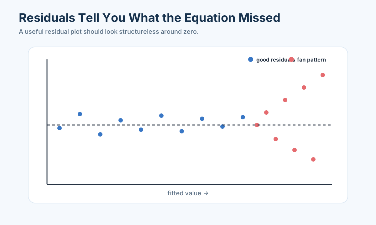
Classical inference usually relies on linear mean structure, zero conditional error mean, independent observations, no perfect multicollinearity, and a justified variance model. Normality is mainly needed for exact small-sample inference, not for defining the least-squares estimate.

Check:

• residual-versus-fitted plot for form and variance;
• QQ plot for severe tail departures;
• VIF or condition number for collinearity;
• leverage and Cook’s distance for influential observations;
• autocorrelation for ordered data;
• train/test performance for generalization.

When variance is unequal, use robust standard errors or model the variance. When observations are grouped or serially related, use an appropriate clustered, panel, or time-series model.

Let the residuals argue with the straight line

Picture a larger apartment dataset. On a residual-versus-area plot, small homes have positive residuals, medium homes negative residuals, and large homes positive again. The line is systematically too low at both ends and too high in the middle; a curved mean function, location mixing, or omitted luxury feature may be involved. The response is not automatically “fit a high-degree polynomial.” First separate neighborhoods and inspect whether the curve persists; then compare a low-order area-squared term or a spline on held-out homes. If the curve vanishes after location is included, the issue was confounding or group mixture rather than a universal physical area law.

Now picture a funnel: residuals are within about 100 rent units for modest homes but spread over 1,000 for expensive homes. Constant error variance is implausible. OLS coefficients can still be a useful summary under certain conditions, but conventional standard errors and one fixed-width prediction interval may be inappropriate. Use heteroscedasticity-robust inference when the mean model is sound, consider modelling variance or using a log response when scale-dependent variation has a defensible interpretation, and evaluate interval coverage separately by rent level. Robust standard errors do not repair a systematically curved mean; a change in variance treatment cannot make the wrong functional form right.

An influential home deserves investigation, not automatic deletion. A 250-square-metre penthouse far beyond most apartment areas has high leverage because its predictor value is unusual. If its rent also deviates sharply, it can pull the fitted slope; Cook’s distance combines residual and leverage to flag that influence. Check whether it belongs to the population being predicted. If a student is budgeting ordinary 40–90-square-metre rentals, excluding penthouses from that target population may be justified with a stated scope. If the city studies the entire rental market, penthouses belong in the data, perhaps as a separate segment. A numerical influence score asks a population question; it does not answer it.

Ordered and clustered observations challenge independence. If ten apartments belong to the same building, they share location, heating, management, and market timing; treating them as ten unrelated draws can make standard errors too small. If rents are recorded monthly, residuals may move together over time as the market changes. Use building-group validation for predicting new buildings, chronological validation for future rents, and clustered or time-aware covariance when inference needs it. The unit of resampling or split should match the unit of generalization, exactly as in the preceding data lesson.

A QQ plot can reveal unusually heavy tails relative to a chosen normal-error reference, but a slight departure in thousands of observations need not be the dominant concern. For exact small-sample classical tests, normality assumptions can matter; for prediction, held-out errors and interval calibration may matter more. VIF or a condition number points to predictors that share information, such as area and room count. None of these diagnostics is a ritual that one performs to earn permission to use OLS. Each asks a concrete question: is mean shape wrong, variance changing, rows dependent, predictors redundant, or a small set of homes steering the result?

The diagnosis should change what we report. If the area-only line has MAE 250 on outer neighborhoods but 700 centrally, one grand MAE conceals who is poorly served. If its residuals show an obvious location pattern, add location or report separate limits. If the fitted mean is reasonable but individual rents vary widely, use a prediction interval instead of pretending the point prediction is a quote. A good regression analysis is not one with no residuals; it is one that can say what residuals remain and how they affect the decision.

Significance and practical importance

Atest asks whether one coefficient is distinguishable from a null value under assumptions. Antest compares a group of restrictions. A p-value is not the probability that the null hypothesis is true and is not a measure of effect size.

Report coefficient, units, uncertainty interval, and practical implication. With enough data, a negligible effect can be statistically significant. With little data, an important effect can remain uncertain.

A small p-value is not a large rent effect

Suppose a large sample estimates an area coefficient of 0.5 rent units per square metre with a tiny standard error, so a test against zero returns a very small p-value. For a 20-square-metre difference, predicted rent difference is only ten units. That may be negligible next to monthly rent uncertainty of hundreds. Conversely a small pilot of twenty apartments may estimate 20 units per square metre but have a wide interval that includes zero; the effect could be practically large yet statistically uncertain. Report estimate, units, interval, and a decision-scale comparison. “Significant” by itself says neither how much rent moves nor whether the estimate supports a budget.

What does a p-value actually ask? Under a specified null hypothesis and model assumptions, it measures how unusual a test statistic at least as extreme as ours would be. It is not the probability the null is true, not the probability a future apartment follows the fitted line, and not a measure of causality. If residuals are strongly clustered by building but the test assumes independent homes, its p-value can be misleading. If we tried dozens of predictors and only show the smallest p-value, selection inflates the chance of a false-looking discovery. Predefine key comparisons or adjust for multiple testing, then validate associations in new data where possible.

An F test compares a group of restrictions, such as whether location and building age coefficients jointly add evidence beyond area under the model. A t test addresses one coefficient. An information criterion such as AIC or BIC balances fit and parameter count under its assumptions; adjustedpenalizes extra predictors differently; cross-validation assesses held-out prediction. These are distinct lenses. If one extra feature improves trainingbut worsens held-out MAE, it may not help a predictive rental tool. If a location coefficient is statistically uncertain but policy-relevant, the right action may be collecting more representative listings rather than declaring “no effect.”

Association language should be precise. “Among observed listings with the same included area and district code, newer buildings were associated with higher rents under this model” is a conditional description. “Renovating an old building will cause its rent to rise by exactly the coefficient” needs causal evidence about who renovates, what else changes, and how market conditions evolve. A student can produce a mathematically correct confidence interval for an association and still overstate it by turning it into a policy intervention claim. The coefficient’s limitations belong next to its number, not hidden in a generic last-page disclaimer.

One way to check practical meaning is to translate a coefficient into a scenario. If estimated retrofit association is -200 kilowatt-hours per month with interval -350 to -50, compare those savings with installation cost, building size, and seasonal variation before recommending an investment. The interval still may reflect confounding, not a causal effect, but it tells us what range the statistical analysis supports under its assumptions. If the decision threshold is -150, the interval crosses it, so one precise recommendation is not yet supported. Effect size and uncertainty should be read together at the action scale.

Nonlinearity and interactions

Linear regression is linear in parameters, so transformed features are allowed:

Use low-order terms supported by plots and validation. An interaction

means the effect ofchanges with. Once an interaction is present, interpret main effects at the reference value of the other variable.

Let the effect change when the context changes

Suppose household electricity use increases with outdoor heat because air conditioning runs. A retrofitted building may respond less strongly. Letbe temperature deviation from a comfortable reference, and letfor a retrofitted building and zero otherwise. Fit. For an unretrofitted building, temperature slope is. For a retrofitted building, slope is. If illustrative coefficients areandkilowatt-hours per month per temperature unit, the retrofitted slope is 12, not -8. The interaction says the difference between slopes is -8. A report that calls“the retrofit effect” without specifying temperature is incomplete.

At, the modeled difference between retrofitted and unretrofitted buildings is. At, it is. Centering temperature around a meaningful reference makesinterpretable; if we used raw Fahrenheit and zero Fahrenheit never occurs in the dataset, the main retrofit coefficient would describe an irrelevant reference situation. The same logic applies to the apartment example: area-by-location interaction lets area slope differ centrally and outside, but the “location effect” then depends on area. State the comparison point whenever an interaction is present.

A quadratic area termcan model curvature while remaining linear in coefficients. But the slope at areabecomes, not one constant number. If the curve was fitted only for 40–100-square-metre homes, it may bend nonsensically at 300 square metres. A spline uses local pieces to control flexibility more cautiously, yet its knots and degrees of freedom must be selected within validation, not chosen after viewing test errors. Plot fitted mean and residuals with observed area coverage; do not let a smooth curve imply support where there are no listings.

Interactions and nonlinear terms should respond to an observed or hypothesized mechanism. If temperature sensitivity differs because of retrofit insulation, the interaction is meaningful. If a dozen arbitrary products of columns improve trainingbut make coefficients unstable, they may be overfit. We can compare a baseline area-and-location model with one justified interaction on held-out buildings or neighborhoods. For causal policy interpretation, even a plausible mechanism needs evidence about selection into retrofit: better-managed buildings may both retrofit and consume less energy for other reasons. Predictive usefulness and causal interpretation remain separate questions.

Logistic and count models

Logistic regression remains linear in the log-odds while producing probabilities between zero and one.

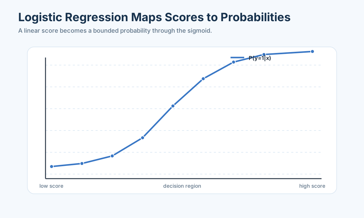
For a binary outcome,

Coefficientchanges log-odds;is an odds ratio. Evaluate probability calibration as well as discrimination. Accuracy alone can be misleading for imbalanced classes; inspect precision, recall, F1, ROC-AUC, and the decision threshold.

For count outcomes, Poisson regression uses. If variance substantially exceeds the mean, investigate overdispersion and negative binomial alternatives.

Classify expensive homes without confusing odds and probability

Suppose a rental site asks whether a listing will exceed a monthly rent threshold. The outcome is binary: expensive or not under a stated threshold. A straight linear regression can predict numbers below zero or above one if used as a probability, especially outside observed feature ranges. Logistic regression maps a linear score through the sigmoid to a value between zero and one. Its coefficient acts on log-odds. If one area coefficient is 0.05 per square metre in an illustrative logistic model, a 20-square-metre difference multiplies conditional odds byholding included features fixed. It does not add 2.72 to probability and does not mean “probability rises by 272%” in every starting situation.

Start with baseline expensive-home probability 10%, whose odds are. Multiplying odds by 2.72 gives odds about 0.302, corresponding to probability. Starting from probability 50%, the same odds multiplier would yield probability about 73.1%. Thus a fixed log-odds coefficient produces different probability differences at different baselines. Translate odds ratios to a few realistic profiles when communicating to a nonstatistical teammate. And remember the conditional association can still be confounded by neighborhood or building quality.

Accuracy can hide class imbalance. If only ten of 100 illustrative listings are above the threshold, a model that always says “not expensive” is 90% accurate but finds none of the ten expensive homes. Suppose another model flags eight, of which six are truly expensive and two are false alarms. Its precision is, recall is, and with 88 true negatives its overall accuracy is. Whether to lower the decision threshold depends on false-positive versus false-negative cost: a budget adviser might prefer not to miss costly homes, while a screening queue may need high precision. ROC-AUC or F1 can summarize discrimination, but the operational threshold and probability calibration still matter.

Calibration asks whether predicted probabilities match frequencies. Among listings assigned about 20% risk, do roughly one in five actually exceed the threshold on held-out data? A model can rank expensive homes well but output probabilities that are too confident; threshold-based financial decisions then fail. Check calibration by group and time, especially if rents shift between seasons. A high area coefficient from a dataset concentrated in one district may not transfer to a new city. We need held-out districts or later months according to the deployment question.

Counts ask for another response model. If the outcome is number of building-service calls per month, Poisson regression connects positive expected counts to predictors through a log link. An illustrative coefficientfor a binary building-age flag would double conditional expected calls under the model, holding included factors fixed. A building observed for two years has more exposure time than one observed for two months, so include an exposure offset or rate definition; otherwise it may look “riskier” simply because we watched it longer. If count variance greatly exceeds its mean or many months have zero calls, diagnose overdispersion or zero-generating mechanisms and compare negative-binomial or other appropriate models. One linear regression family does not fit every outcome support.

Regularization

Ridge regression minimizes

shrinking correlated coefficients. Lasso usesand can set coefficients to zero. Standardize predictors and chooseby validation. Feature selection must occur inside the validation procedure.

We have distinguished statistical significance from a practically useful effect. A decision-maker still needs to know how uncertain a new prediction is, not merely how precisely we estimated the average relationship.

Correlated features make a coefficient contest unstable

Suppose a housing dataset has floor area, room count, and building footprint. Larger homes usually have more rooms and larger footprints, so these predictors may move together. An ordinary least-squares fit can predict rent reasonably while assigning one month a large positive coefficient to area and negative one to room count, then reversing them when a few listings change. The combined prediction may stay similar even though individual coefficients are unstable. If the goal is to explain the price of one extra room while holding area fixed, we need enough homes with different room counts at comparable area; otherwise the data do not identify that separate effect well. Regularization can stabilize prediction, but it cannot manufacture missing comparisons.

Ridge adds a squared-coefficient penalty. It pulls large coefficients toward zero and can distribute weight among correlated predictors rather than letting one dominate arbitrarily. Lasso adds an absolute-value penalty and can set some coefficients exactly to zero, producing a smaller feature set. These penalties change the objective: we accept a little more training residual error to improve stability or held-out performance. The strengthmust be chosen on training folds, not after seeing final test errors. Feature scales matter because a coefficient measured per square metre and one measured per thousand currency units face different raw penalty magnitudes. Standardize within each training fold, then explain predictions or coefficients in meaningful original units.

Consider a two-feature toy example: area in square metres and the same area converted to square feet. They are almost exact duplicates. Lasso may pick one and drop the other, but which one survives can change with preprocessing or tiny data changes. It would be wrong to claim the selected unit “causes rent” while the dropped unit has no relationship. Ridge may keep both with smaller values, but individual coefficients are still hard to interpret. Remove known duplicates using the data dictionary first. Penalties should respond to remaining correlated information, not substitute for source understanding.

Variable selection itself can leak. Suppose we inspect every column’s correlation with rent on the entire dataset, keep the top five, and then perform cross-validation only on the ridge model. The test folds influenced which columns were chosen. Put selection inside each training fold or predefine features from domain knowledge before splitting. Nested tuning is useful when comparing many choices; a late untouched test set should remain untouched through method selection. A lasso model with 99% trainingbut poor later-building error has not earned a simpler narrative merely because it outputs sparse coefficients.

Regularization has a different role when causal interpretation is the goal. Shrinkage deliberately biases coefficients toward zero, and automatic selection can obscure confounders. A policy question about whether retrofits reduce energy use needs a defined comparison, confounder strategy, and uncertainty analysis; predictive ridge or lasso performance alone cannot answer it. We can still use regularized models as predictive baselines or as exploratory tools, but label their claim. “This feature helped held-out prediction” is not “changing this feature would change the outcome.”

Prediction uncertainty

A future individual observation contains both mean-estimation uncertainty and irreducible outcome variation, so its interval is wider.

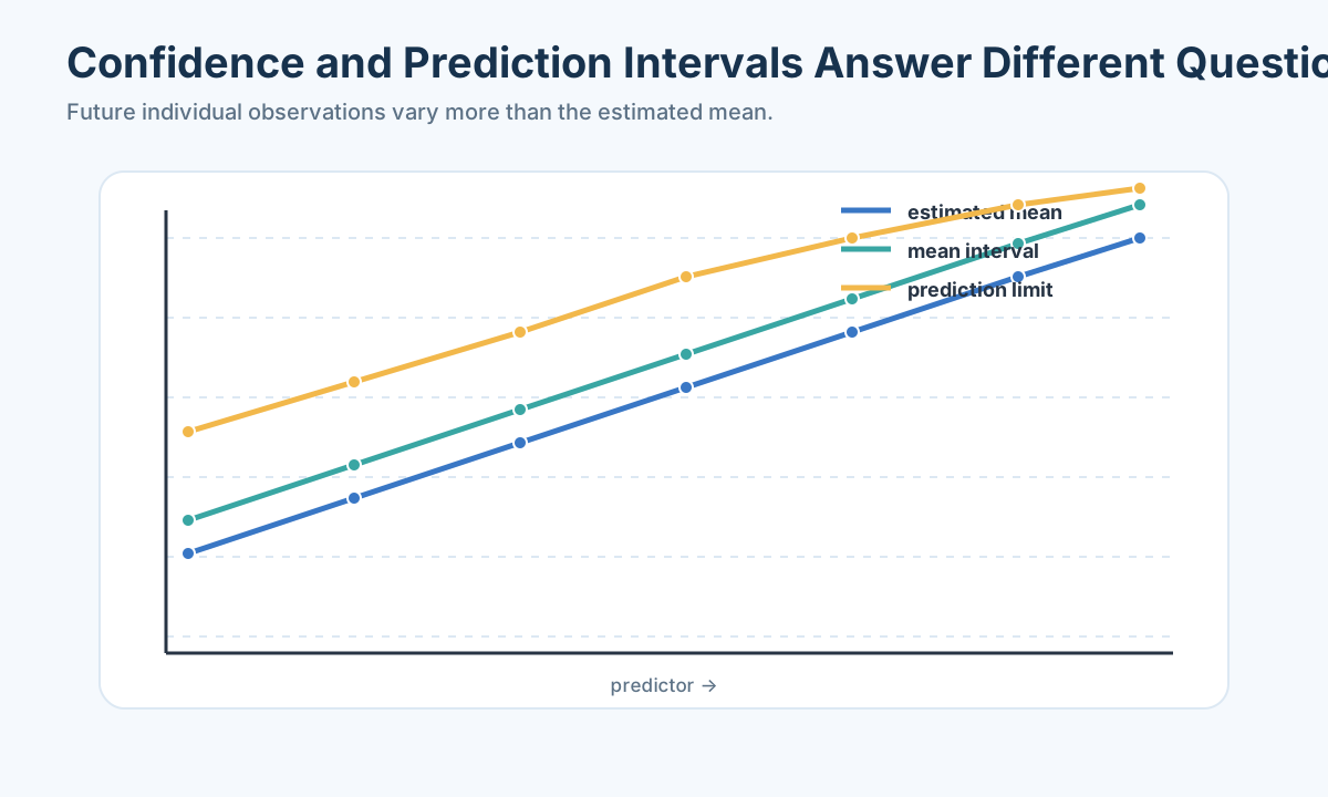
A confidence interval estimates uncertainty in a conditional mean; a prediction interval covers a new individual observation and is wider. Report held-out MAE or RMSE and interval coverage. Use chronological validation for time-dependent observations.

The interval around one apartment is wider for a reason

Return to the four-apartment line. At 80 square metres it predicts 2,000 rent units. A confidence interval for the mean rent of all comparable 80-square-metre apartments under the model reflects uncertainty in the fitted line. A prediction interval for one new 80-square-metre apartment must add the spread among individual homes—the two observed 70-square-metre homes already differed by 200. Even if we measured thousands of homes and knew the average line very precisely, individual rents could still vary with unmeasured condition and bargaining. That is why the individual prediction interval stays wider than the mean confidence interval. A tenant needs the latter only if they ask about average markets; for a specific listing budget they need the former.

Do not invent a narrow interval from four toy homes. With so little data, variance and model shape are poorly known, and the four listings may not be representative. On a real larger dataset, calculate an interval under stated residual assumptions and check held-out coverage by area and district. If nominal 90% intervals contain only 60% of actual central-home rents, the location structure or variance model is wrong for that group. A bootstrap can help estimate uncertainty, but resample buildings rather than individual apartments if many listings share a building; use time blocks for monthly data. The resampling unit follows the data-generating unit.

The distinction persists for binary probabilities. Logistic regression may estimate that homes in one profile have 23% chance of exceeding the threshold. An interval around that estimated probability reflects model and sample uncertainty; whether one particular home exceeds threshold is a Bernoulli outcome with its own irreducible unpredictability. Calibrate predicted probabilities on held-out groups. A confident 23% from an unrepresentative sample is not a good risk estimate. Probability uncertainty and individual outcome uncertainty are separate layers.

We should also compare a prediction interval with the decision threshold. Suppose a renter can afford at most 2,200 monthly units. A point forecast of 2,000 appears affordable, but a plausible prediction range of 1,600–2,700 crosses the budget line. The appropriate conclusion is not simply “rent will be 2,000”; it is that area alone does not settle affordability for a specific listing. Request neighborhood, building condition, and actual asking price before committing. Regression can guide a search or screening decision without pretending to replace the final observation.

The next fitting choice follows the purpose

For a rental budget, area-only OLS is an honest baseline. Location and age may improve held-out accuracy; a justified interaction may correct slope differences; ridge may stabilize correlated housing features; a tree may capture a local threshold. Give each method the same held-out buildings or later listings, depending on deployment, and score MAE and interval coverage. If a tree wins prediction but cannot support an interpretable area association, use it for prediction while keeping a separate, carefully conditioned explanatory model for discussion. “One best regression” is not a universal idea when goals differ.

A compact implementation separates training and test data before fitting preprocessing:

from sklearn.compose import ColumnTransformer
from sklearn.impute import SimpleImputer
from sklearn.linear_model import Ridge
from sklearn.metrics import mean_absolute_error
from sklearn.pipeline import make_pipeline
from sklearn.preprocessing import OneHotEncoder, StandardScaler

numeric_columns = ["area_m2", "building_age_years"]
categorical_columns = ["district"]
numeric = make_pipeline(SimpleImputer(strategy="median"), StandardScaler())
categorical = make_pipeline(
    SimpleImputer(strategy="most_frequent"),
    OneHotEncoder(handle_unknown="ignore"),
)
prep = ColumnTransformer([
    ("num", numeric, numeric_columns),
    ("cat", categorical, categorical_columns),
])
model = make_pipeline(prep, Ridge(alpha=1.0))
model.fit(X_train, y_train)
pred = model.predict(X_test)
print(mean_absolute_error(y_test, pred))

The pipeline ensures that imputation, scaling, and encoding learn only from the training set.

Verify one transformed listing rather than trusting the pipeline name

The code assumes X_train and X_test were split in a way that matches deployment. If we want to predict rents in unseen districts, a random listing split may leave the same district in both groups and overstate transfer; holding out districts is a tougher and more relevant check. If the task is future listings in existing districts, use a chronological split. The pipeline prevents its imputer, scaler, and encoder from fitting on test rows after the split, but it does not choose a correct split or prevent an illegal future feature from appearing in X_train. “Leakage-safe pipeline” is a claim about the transformation boundary, not the whole project.

Pick one test apartment with area 80 square metres, building age missing, and district “north.” Suppose the training median age is 20 years. The numeric imputer inserts 20 and the scaler uses training means and standard deviations, not test values. The one-hot encoder maps north to the district column learned in training; if north was unseen, handle_unknown="ignore" produces all zeros for that categorical field under this particular encoding, which may not be an adequate representation of a genuinely new district. The model still predicts a rent, but we should flag and test how it behaves for unseen locations. An implementation can be technically valid and operationally weak outside its training category support.

The selected Ridge(alpha=1.0) is a demonstration value, not a tuned conclusion. Compare several penalty strengths using inner training folds, keep the final test set untouched, and check error by district and rent range. A pipeline can support cross-validation by refitting transformations inside every training fold, which is its major advantage over preprocessing the full table once. Still define the response, feature dates, units, category meanings, and grouping before passing rows into it. A ten-line implementation cannot establish a causal rent effect; it can only implement one predictive workflow under a data contract.

The output MAE has the unit of y_train and y_test, so if rent is monthly currency units, report it as such. Do not compare a MAE of 250 in one currency with 250 in another without conversion. If one district’s error is 800, a global 250 may not characterize that district’s users. Also record how many test rows had imputed age and how many carried unseen districts, so readers know where the pipeline relied on fallback rules. A prediction table with actual rent, predicted rent, residual, and key subgroup flags is more informative than one scalar printed by the code.

From association to prediction

Suppose we model household electricity consumption using floor area, occupants, building age, temperature, and retrofit status. Start by deciding the goal. Explanation asks how consumption changes with a predictor under assumptions; prediction asks how accurately new households can be estimated. The same regression can serve either goal, but validation and language differ.

Read a coefficient conditionally

In

is the expected difference associated with one unit of area holding occupants and temperature fixed. It is not necessarily the causal effect of constructing a larger home. Omitted income, building type, or behavior may confound the association.

Center continuous variables when interactions are present. With, whereindicates retrofit, the temperature slope iswithout retrofit andwith retrofit. Main effects cannot be interpreted without the interaction.

Diagnose assumptions visually

Plot residuals versus fitted values for nonlinearity and unequal variance, a Q–Q plot for tail behavior when inference relies on normal errors, residuals versus time for dependence, and leverage/Cook’s distance for influential observations. A significant coefficient does not rescue a misspecified model.

Transformations should follow mechanism. A log response turns additive coefficients into approximate percentage changes and can stabilize multiplicative noise. Polynomial terms approximate curvature but extrapolate dangerously. Splines give local flexibility; specify knots or degrees of freedom and validate them.

A log response changes the question’s scale

Suppose energy consumption varies more in large buildings than small ones, roughly proportionally to their level. Instead of modelling monthly kilowatt-hoursdirectly as an additive line, we might modelfor positive. A coefficientper square metre on the log scale means a one-square-metre increase is associated with approximately 1% higher conditional energy, and an exact multiplicative factor ofunder the specified model. For a 20-square-metre difference, the factor is, not “20 extra kilowatt-hours.” Coefficients must be interpreted on the scale actually fitted.

Why might this help? If variation is about 10% of consumption at all sizes, a raw-scale residual plot will fan outward asgrows; log-scale residuals may have a more even spread. But logs cannot handle zero or negative energy values without a separate convention, and a zero may be a genuine closed month, a meter outage, or an import error. The correct handling follows the measurement story. Also, exponentiating a predicted mean log energy does not in general give mean energy when residual uncertainty exists; it is closer to a median under common assumptions. If the budget needs expected kilowatt-hours, account for back-transform bias and validate on the original scale.

Splines offer another kind of flexibility without changing outcome scale. Suppose outdoor temperature has a comfort region where energy use stays low, then rises in hot weather due to cooling and in cold weather due to heating. One straight temperature slope cannot represent both directions; a quadratic term may approximate a U shape, while a spline can form local slopes across temperature ranges. The data must cover both cold and hot ranges, and knot positions or degrees of freedom must be chosen from training data and validated on later buildings. A perfectly smooth fitted curve at unprecedented 45-degree weather is still extrapolation beyond support.

For a rental example, an area-squared term might imply diminishing or increasing rent per extra square metre. Check whether it persists within neighborhoods instead of arising from luxury units at the high end. If the apparent curve disappears after building type is included, reporting a universal “nonlinear area law” would overstate the evidence. Plot predicted mean, observed points, and residuals by group. A transform or nonlinear term is a proposal about mechanism and scale, not just a way to lower the training loss.

Finally the model must return to the decision’s unit. A student comparing OLS on raw kilowatt-hours with a log-response model should score both on held-out kilowatt-hours and show interval coverage in those units. If one model has low log-scale error but underpredicts peak consumption, it may be unsuitable for capacity planning. The choice is evaluated at the question’s scale, not the software’s convenient transformed scale.

Distinguish uncertainty types

A confidence interval quantifies uncertainty in an estimated parameter or mean response under the model. A prediction interval adds individual variation. Bootstrap intervals can help when analytic approximations are doubtful, provided resampling respects clusters and time.

Multiple testing inflates false discoveries. If dozens of coefficients are screened, control family-wise error or false discovery rate, or treat the analysis as exploratory and validate on new data. Report effect size and interval, not only a p-value threshold.

Expand to generalized models

Binary outcomes use logistic regression:

Exponentiating a coefficient gives an odds ratio, not a probability difference. Counts may use Poisson or negative-binomial regression with an exposure offset. Proportions, durations, and zero-inflated outcomes require distributions consistent with their support.

A model can be accurate overall and poor for one neighborhood

Imagine our rental model is tested on 100 later listings: 80 are ordinary outer-neighborhood homes and 20 are central homes. It has MAE 200 rent units on the outer 80 and MAE 800 on the central 20. Overall MAE isunits. That one number looks respectable until a central renter uses it: their expected absolute error is four times as large as for an outer renter. If the model systematically underpredicts central rents, a budget decision can fail. Report error by district, rent level, area range, and listing date. Subgroup diagnostics should match the people or buildings the tool will actually serve.

Why might this happen? Central homes could differ in amenities not recorded in the training table. Their rents may change faster after a new transit connection. The training set may contain few central listings; an area coefficient learned mainly from outer homes is extrapolated into a different market. A tree may make a better central split if it has enough examples, but with only a handful it can overfit. More representative listings, better condition features, a district-specific baseline, or a wider central prediction interval may be more valuable than another algorithm. Diagnose data support before tuning complexity.

Validation can also hide similarity. If two apartments in the same building are nearly identical, splitting them across train and test produces easy predictions that do not show whether the model works for a genuinely new building. Group by building for that deployment. If the objective is future listings in buildings already on the platform, a chronological split may be relevant instead. If rents changed after a policy shock, random rows from before and after in both sets let the model use later market levels when “predicting” earlier listings. The evaluation claim should say what is new: home, building, neighborhood, or time.

Probability classification has the same subgroup issue. Suppose the expensive-home classifier’s overall predicted 20% probabilities calibrate well, but central listings assigned 20% exceed the threshold 40% of the time while outer ones do so only 15%. A threshold rule based on the global 20% is miscalibrated centrally. Recheck labels and sample representation, recalibrate or remodel by group where evidence supports it, and report uncertainty. A discrimination score like ROC-AUC may still look good globally while the probabilities used in decisions fail for one important group.

Fair evaluation should not be confused with guaranteeing identical error for every group at any cost. Some groups may genuinely be harder to predict because the table lacks relevant measurements or the market is more volatile. The first duty is to reveal those differences, explain their likely sources, and avoid presenting one global interval or MAE as if it applied everywhere. Where uncertainty is wider, use a wider interval or collect better data; where systematic bias is visible, test whether a mechanism-supported feature can correct it. A regression model is an estimate with a scope, not an oracle for every row sharing a column name.

Compare machine-learning models fairly

Regularized linear models provide stable baselines. Trees capture thresholds and interactions; random forests reduce tree variance; boosting builds sequential corrections; kernel methods capture nonlinear geometry; neural networks are useful when data volume and structure justify them. Tune every candidate inside training folds and evaluate once on untouched test data.

Use permutation importance or accumulated local effects cautiously when interpretation matters. Feature importance is not causality, and correlated predictors can split or hide importance. Calibrate probabilities for decisions based on risk thresholds.

Two honest conclusions from the same energy table

Suppose the team has monthly energy records for 200 buildings over three years. An explanatory analysis asks whether retrofit status is associated with different consumption after accounting for area, weather, occupancy, and building type. It reports a conditional coefficient, interval, residual checks, and a limit about selection into retrofit. It might keep confounder-related features even if they barely improve prediction, because removing them changes the comparison being described. A predictive analysis asks how accurately next winter’s consumption can be forecast for buildings not yet observed in winter; it chooses features and tuning by held-out building and time performance, and reports individual prediction intervals and peak-month errors. The two analyses can use the same table but should not silently share one “best” model.

Imagine the explanatory OLS model estimates retrofitted buildings use 180 fewer kilowatt-hours per month, with interval from -300 to -60 under its error and sampling assumptions. This is not yet a causal payback estimate. If retrofits were chosen for buildings whose managers also changed thermostats, the coefficient may mix effects. The predictive ridge model might have lower later-building MAE, perhaps 95 versus 120 kilowatt-hours, but shrink the retrofit coefficient toward zero; that does not disprove the association estimate either, because ridge optimized a different objective. A tree could predict best yet offer no single conditional retrofit slope. Each output is read under the question it was built to answer.

For the explanatory report, show before/after patterns, compare similar building groups, examine weather and occupancy changes, and state what design would strengthen a causal claim. For the predictive report, show area-only and weather-only baselines, split by building for transfer, split by time for next-winter conditions, inspect errors by building type and season, and test whether intervals cover peak months. If the flexible model depends on actual future weather rather than archived forecasts, repair the validation before reporting its lower MAE. If the explanatory interval relies on independent rows while each building contributes dozens of months, use building-cluster-aware inference or revisit the model.

The student can then write two concise sentences: “Under the observed covariates, retrofit status is associated with lower energy use, but this comparison may be confounded by management and selection”; and “For next winter, the selected predictive workflow has this held-out error and this uncertainty under forecasted weather.” Neither sentence needs to claim that one result proves the other. If the policy goal is payback, plan an intervention comparison; if the goal is capacity, use the prediction and stress scenarios. This is how regression becomes a tool for a real question rather than a single table of coefficients.

Regression sequence from the course

Start with descriptive plots and a baseline. Pearson correlation measures linear association, Spearman rank correlation monotone association; neither adjusts for confounding or proves causality. A heat map is a screening tool, and highly correlated indicators may double-count information in later evaluation models.

For, OLS iswhen full rank holds. Interpretas the change in conditional mean per unit of, holding included predictors fixed. The t-test evaluates one coefficient, the F-test a group, and adjusted, AIC/BIC, cross-validation, and residuals answer different model-selection questions.

Residual plots check linearity, constant variance, influential observations, and structure left unexplained. Heteroscedasticity-consistent standard errors repair inference under some variance misspecification but do not repair a wrong mean function. Clustered or time-dependent errors require corresponding covariance or model structure.

Training fit and future prediction pull in different directions

Suppose a degree-one area model has training MAE 300 rent units, degree-two has 250, and degree-six has 80. It is tempting to announce degree-six “best.” Now hold out apartments from a later season or a different neighborhood and find MAEs 330, 310, and 900 respectively. The degree-six curve followed historical quirks and extrapolated poorly; its spectacular training fit was not a forecast success. AIC or BIC would penalize some extra complexity under model assumptions, but they cannot replace the held-out setting that matches deployment. If the city wants to predict rents in new neighborhoods, validation must hold out neighborhoods; random listing rows may leave near-identical buildings in both parts and flatter the complex curve.

An adjustedcan help compare linear models while accounting for predictor count, but it still measures explained variation within the selected sample and assumptions. A residual plot asks whether the mean structure is wrong. A t test asks whether one coefficient differs from a reference under an inferential model. Cross-validation asks whether new cases are predicted more accurately under a split. These tools can disagree without contradiction because they ask different questions. If degree-two improves held-out error and residual curvature, it has stronger evidence for a predictive housing baseline than degree-six’s training.

The choice also depends on what is being estimated. For an explanatory report about area association, an interpretable line plus district effects and an honest interval may be useful even if a tree has lower MAE. For a search site’s listing-price recommendation, the tree’s predictive gain could be worthwhile if it generalizes and its errors by neighborhood are acceptable. For a retrofit policy, neither high predictive accuracy nor a small p-value alone establishes causality; the study design must address how buildings entered the intervention group. One dataset can support several models, each serving a distinct claim. Presenting them as one winner-takes-all contest obscures the goal.

We can also be underfit. If both training and held-out errors are high and residuals show a clear temperature threshold, an area-only linear model lacks important structure. Add one mechanism-supported term and retest. If training error falls sharply while held-out error worsens, added complexity is suspect. If both improve and residual structure diminishes, the new feature has earned its place. This progression—baseline, diagnosed failure, limited extension, common validation—is what a skeptical teammate can follow. It is more informative than listing every algorithm the library offers.

Nonlinearity, classification, and regularization

Add interactions when one effect depends on another:. Centering can make main effects interpretable. Splines represent smooth nonlinear response with controlled flexibility.

Logistic regression models

sois a conditional odds ratio. Evaluate discrimination and calibration; accuracy is misleading under imbalance. Ridge minimizes RSS plusand stabilizes correlated coefficients. Lasso usesand can select variables, but selected sets may be unstable.

Prediction uncertainty

A confidence interval foris narrower than a prediction interval for a new. Bootstrap when analytic assumptions are doubtful, preserving groups or time blocks. For black-box models, use nested tuning, subgroup errors, calibration, and permutation tests. Feature importance is association with predictive performance, not causal effect.

The course sequence introduced fitting, diagnostics, and interpretation separately. This complete case lets us connect them: choose a response, fit a baseline, inspect what failed, and explain what can be predicted responsibly.

Worked case: building energy

Suppose a campus team wants to estimate next winter’s monthly electricity consumption for residential buildings, then asks whether retrofitting insulation might reduce that consumption. Those are related but different questions. The first is prediction under anticipated weather and occupancy. The second is an intervention effect: what would the same building consume if it were retrofitted versus not, with other conditions comparable? A predictive regression might use building type, area, and neighborhood effectively while still fail to establish the second claim because buildings chosen for retrofit may differ before treatment. We will make the prediction first and keep the policy wording cautious.

Take three illustrative monthly building records to see the measurements. Building A has 100 square metres, two occupants, and 300 kilowatt-hours; B has the same area, four occupants, and 400 kilowatt-hours; C has 150 square metres, two occupants, and 450 kilowatt-hours. These values do not give enough data for a real fit, but they tell us area alone cannot explain A versus B. Occupants, weather, appliance use, heating system, and building type may matter. If one record says 300 kilowatts instead of kilowatt-hours, it describes power rather than monthly energy and should not be merged into the response column. Confirm meter interval, unit, and whether common-area energy is included before fitting.

Start with an area-only baseline on training buildings. Plot energy against area and residuals by occupancy and winter temperature. If high-occupancy buildings have consistently positive residuals, add occupancy as a candidate predictor. If residuals curve with outdoor temperature, a heating or cooling threshold may be more realistic than one straight slope: consumption can remain low near comfort temperature and rise when it gets very cold or hot. A spline or piecewise term can capture that pattern within the observed temperature range; extrapolating it into record cold should be stress-tested, not presented as certainty. Add a building-type interaction if the same temperature shift affects old masonry and modern insulated buildings differently.

For predictive validation, hold out whole buildings if future deployment includes new buildings. If we randomly split monthly rows from the same building, training sees its stable features and test sees a later month of a familiar building; that may be a valid test for future months of known buildings but not for transfer to unseen ones. If the target is next winter, also use chronological origins so the weather forecast and occupancy plan available before each month are the inputs. Compare area-only OLS, area-plus-occupancy OLS, ridge, and perhaps a tree under the same split. Report MAE in kilowatt-hours, error by season and building type, and whether prediction intervals cover later energy use.

Suppose the flexible tree has lowest held-out MAE but responds erratically to temperature outside training range. Ridge may be slightly less accurate overall and more stable under winter stress. The choice depends on whether the downstream decision is annual budgeting, monthly supply capacity, or identifying unusual buildings for an energy audit. A prediction error of 50 kilowatt-hours on a quiet month may matter less than underpredicting a peak heating month by 500. Test the model against the budget or capacity decision, not only one averaged error. A fallback model should be available when next month’s weather forecast is missing.

Now return to the retrofit question. If retrofitted buildings in the observed dataset use 200 fewer kilowatt-hours per month after adjustment, we can say they are associated with lower use conditional on included area, occupancy, weather, and type. We cannot yet say retrofitting caused 200 savings. Perhaps buildings with proactive managers retrofit and also fix thermostats; perhaps residents changed; perhaps retrofit timing coincided with mild weather. A credible intervention estimate needs a design such as comparable before/after building histories, appropriate controls, and checks for other simultaneous changes. Keep predictive model selection separate from this explanatory evidence. A low MAE for a retrofit predictor does not turn its coefficient into a causal return-on-investment estimate.

The final student report should therefore give two outputs if both questions matter: a forecast and interval for next winter’s energy by building, with held-out error and inputs, and a limited statement about retrofit association plus what additional comparison is needed for causality. This is more useful than one impressive regression table. The model can guide an energy audit even if it cannot yet support a financial payback claim. It can identify high-use buildings where measurement or intervention study would be valuable, while honestly stating the uncertainty about why they use more.

What would move a retrofit association toward a causal question?

The building case left a practical question open: if retrofitted buildings use less electricity, did the retrofit cause the reduction? Suppose treated building T used 500 kilowatt-hours in a comparable pre-retrofit month and 400 afterward, a raw decline of 100. Control building C, not retrofitted, used 450 before and 420 afterward, a decline of 30. A simple difference-in-differences comparison iskilowatt-hours. It subtracts a change that also happened without retrofit, perhaps because weather was milder. This is a supplementary teaching calculation, not a claim the lecture deck provides a full causal-inference course.

The -70 estimate still relies on assumptions. Were buildings T and C on roughly parallel trends before the intervention? Did occupancy, equipment, or meter definitions change in T but not C? Was the control building comparable in heating system and exposure to weather? One before and one after month are far too little to check parallel trends or seasonal effects. We would collect multiple months, match comparable buildings, adjust for weather and occupancy without conditioning on variables changed by the retrofit, and inspect pre-intervention trends. A regression can express the comparison more systematically, but its coefficient will inherit the study design’s limitations.

This example distinguishes three claims with the same numerical vocabulary. An area coefficient in OLS is a conditional association. A held-out energy forecast is a prediction. The treated-versus-control contrast is an attempt at a causal effect under a design and assumptions. They can use regression algebra, but the evidence needed differs. If someone says “ridge had the lowest MAE, therefore retrofit will save 70 kilowatt-hours,” they have jumped from prediction to intervention without a bridge. The correct next step is an intervention study, not a stronger predictive algorithm.

The same reasoning applies to rents. Listings near a new station may be more expensive after it opens, but perhaps those neighborhoods were already on a rising trend. A before/after comparison with comparable areas can help, yet changes in zoning, development, and renter mix may still confound. A student paper should phrase what is supported—association or a design-dependent causal estimate—and what remains untested. Being precise about claim type is a form of mathematical honesty.

A rental budget is not a fitted coefficient table

Imagine a student deciding whether an 80-square-metre apartment is within a monthly budget of 2,200 currency units. Our four-home area-only fit predicts 2,000, but it cannot tell whether the actual apartment is in an expensive central district or has unusual amenities. A useful search tool would combine area with verified location and condition features, estimate a prediction range for an individual listing, and flag whether the home lies within the training distribution. If the predicted range crosses 2,200, the model should say the budget decision is unresolved, not print “affordable” because its mean is 2,000.

Suppose a richer model predicts 2,150 with an illustrative individual interval 1,750–2,650. The range does not claim every apartment at 80 square metres can cost exactly these endpoints; it expresses model and outcome uncertainty under a particular calibration. The student can use it to prioritize listings for inspection but must still read the actual asking rent and contract terms. If the model’s interval undercovers central listings, its “budget-safe” label is especially risky there. In the report, show held-out coverage by district and one example of a wrong budget decision, not only the average prediction error.

There is a second question the student might ask: “Would choosing a 60-square-metre place instead save about 20 times the area slope?” The toy area-only slope predicts a 300-unit difference, but that is a conditional model comparison only if the homes are otherwise similar under included features. Smaller apartments could be concentrated in different neighborhoods, have higher rent per square metre, or be newer. An area-by-district interaction could make slopes differ, and a nonlinear model could make marginal rent vary with size. If the student compares two actual listings, their asking rents are more informative than multiplying a pooled coefficient. The regression helps frame expectation and uncertainty; it does not erase known prices.

For a housing policy paper, a coefficient may be used to describe a pattern across the market, but the estimand must be named: conditional rent difference by area within included district groups, not the causal return from constructing more space. If city council asks whether building smaller units would reduce rents, supply, zoning, and selection mechanisms are part of the intervention question. A predictive rental calculator and a causal housing policy claim may require separate models or evidence. Reporting these distinctions to a beginner is not an academic ornament; it prevents a tidy slope from becoming a false recommendation.

This one student story touches most of the lesson: response and unit, baseline least squares, residual spread, location confounding, interactions, subgroup validation, individual interval, and action threshold. The reader can see why each tool enters because the budget question becomes sharper at each step. A long statistical table without this link would be less useful even if all its standard errors were calculated correctly.

Explain one regression result without hiding the limits

Suppose a team presents the building-energy model to a campus facilities manager. The first sentence should state the target and horizon: monthly electricity use in kilowatt-hours next winter for buildings not yet observed under next winter’s weather forecast. Then give the held-out building-group error, interval coverage, and the difficult regimes—perhaps very cold months and older building types. If the selected model needs occupancy plans and weather forecasts before each issue date, say when those inputs arrive and what fallback is used if they do not. A manager can then decide whether the forecast is precise enough for supply planning. A list of coefficients without these conditions will not answer the operational question.

For the explanatory retrofit analysis, use different words: “Retrofitted buildings in our sample had an estimated conditional difference of this many kilowatt-hours after adjusting for measured area, weather, occupancy, and type.” Show the interval and note building-clustered observations if each building contributes months. Then say why the association may not equal savings from performing a retrofit—selection, other management changes, and pre-existing trends. The supplementary treated-control hand example showed one possible design, but one before and after month is insufficient evidence for a causal claim. The facilities manager should not budget retrofit payback directly from a predictive ridge coefficient.

A good figure can carry much of this story. Plot observed versus predicted energy by building type with units, and mark peak winter months; a residual plot shows where the mean is systematically wrong. For rent, plot the area-only line with observed apartments colored by district, plus an individual prediction band where supported. Do not fill the band beyond the observed area range as though penthouse predictions were as certain as ordinary homes. Put one sentence under each figure stating the pattern it tests: missing district effect, variance funnel, or interval undercoverage. The reader should know what belief each plot challenges.

When reporting a coefficient, include reference profile and scale. “Area coefficient 15” is incomplete: 15 monthly rent units per square metre under the area-only line, with a toy sample and no location control, is a usable description. “Retrofit interaction -8” is incomplete unless we say it is the difference in temperature slopes between retrofit groups under our centered temperature reference. “Logistic area coefficient 0.05” acts on log-odds per square metre; for a 20-square-metre change, conditional odds multiply by. Translations like these prevent correct algebra from being misread as a probability change or causal cost.

Finally show a version of the model that failed and what was learned. Perhaps the area-only rent line underpredicted central homes; adding district improved some held-out groups. Perhaps degree-six area curve fit training homes almost perfectly but failed on a later neighborhood. Perhaps a nominal 90% interval covered only 60% of peak winter energy uses. These failures reveal why the chosen extension and uncertainty statement exist. A modeling paper becomes persuasive when another team can reconstruct the baseline, inspect the diagnostic, and see that each added term responds to evidence rather than to a desire for a more impressive formula.

All apartment rents, building electricity values, classifier counts, log-scale coefficients, and treated-control differences here are invented teaching numbers. They demonstrate calculation and interpretation, not real market or retrofit estimates. The technical method topics follow the course deck; any application requires a sourced dataset, justified split, and checked assumptions. The next lesson will turn to a situation with no predefined response variable, where clustering and dimension reduction describe structure rather than predict a chosen outcome.

To make interval language tangible, imagine a larger, properly validated rental dataset where estimated average rent at 80 square metres is 2,000 with illustrative mean interval 1,950–2,050, while individual listings at that profile have an illustrative prediction interval 1,600–2,400. These numbers are not derived from our four-home toy fit. The first says the average line is estimated with modest uncertainty; the second says real individual homes differ widely even at the same measured profile. If a student has a maximum budget of 2,200, the mean interval lies below it, but the individual interval crosses it. Reporting only the narrower mean interval would give false comfort for one apartment search.

Now suppose a central district’s held-out listings routinely sit above 2,400. The global individual interval is under-covering that group. We should not widen the interval for all homes reflexively before checking whether an omitted district feature or subgroup-specific variance explains the pattern. If the area-and-district model removes bias but central outcomes remain more variable, use an appropriately wider central interval and report its later coverage. The interval is a model output to validate, not a decorative ribbon around a line.

The same uncertainty distinction affects retrofit claims. An interval for the conditional association coefficient says how precisely that coefficient was estimated under the statistical model, not how variable one building’s energy use will be next month and not whether retrofitting that building will causally save the interval’s midpoint. A prediction interval for next month’s building energy answers another question. A causal effect interval would require an intervention design. Readers should be able to match each interval to its underlying quantity, population, and assumptions before using it for a decision.

One final test of communication is to hand the model summary to a teammate who did not fit it. Ask them whether “area coefficient 15” applies to a central penthouse, whether “retrofit coefficient -180” proves a payback, and whether the narrow average-rent interval is the right range for one listing. If they answer yes to all three, the report needs clearer scope, design, and interval labels. A model can have correct code and misleading prose. The goal is for a reader to identify the supported comparison, the extrapolation boundary, and the decision-relevant uncertainty without having to reverse-engineer the notebook.

This is why the lesson began with four apartments rather than a package output. The hand calculation exposed what the fitted line does and what it leaves behind. Every extension afterward had a reason: location addressed a subgroup difference, an interaction addressed changing slope, regularization addressed instability, logistic and count links matched outcome support, and interval checks addressed decisions about individuals. The sequence is reusable. In a new dataset, start with one small worked row and one honest baseline, then let residuals, group coverage, and the actual question determine what structure to add.

That is the practical habit I want you to keep.

Regression assigns a role to an outcome variable. When we do not yet have such a target, the next lesson asks a different question: what structure can we find among the observations without pretending that a cluster name is a prediction?