Mathematical Modeling 13 - Forecasting Models

Last lesson cleaned and diagnosed a time series. Now the restaurant manager wants to order food for next week. How many lunches should she prepare tomorrow, and how uncertain is that number? A forecast is valuable only when it improves that decision, not when its plot happens to follow the past smoothly.

We will start with forecasts a beginner can calculate—last value, seasonal repeat, and smoothing—then ask when ARIMA, volatility, grey models, or regression add something. Every method will face the same future periods and a plain baseline. We will also distinguish predicting an average from predicting a range: ordering 120 lunches when demand might be anywhere between 80 and 170 is a different decision from ordering 120 under a narrow range.

Forecasting is model comparison under a time-respecting protocol. Start with a baseline, add structure that is visible and defensible, and keep the simplest model whose out-of-sample behavior supports the decision.

Smoothing models

A moving average reduces short-term variation but delays changes. Simple exponential smoothing updates level by

Holt’s method adds trend; Holt–Winters adds seasonality. These models are strong when the series is driven by evolving level, trend, and seasonal components rather than rich lag interactions.

Smoothing is a simple answer when recent observations carry most of the useful information. ARIMA asks a sharper question: does the error left after accounting for trend and past values still have predictable structure? We will connect that question to the model terms.

Forecast with a pencil before choosing a package

Suppose our lunch-box shop sold 100, 120, 125, 130, and 135 boxes over five comparable ordinary days. A last-value forecast for tomorrow is 135. A three-day simple moving average is. Neither is inherently superior. The last value reacts quickly to a real upward change but also reacts to a one-day accident; the three-day average reduces noise but lags behind a sustained rise. If the next observation is a promotion spike of 190, the last-value method will forecast 190 for the following ordinary day unless we label the event, while a moving average will remain partly inflated for several days. Smoothing changes the weighting of history; it does not identify the event’s cause.

Simple exponential smoothing makes the weights implicit in a recursive level. Letand. When the next observed value is 120, updated level is. With the following 125, it becomes. The one-step forecast after that is 114.8 in this toy setup. This lags the rising data because it discounts recent change. Ifwere near one, it would track the latest observation closely; if near zero, it would move slowly. The weights on older data decrease geometrically: expand the recursion once or twice to see current value weighted by, previous by, and so on. We can fiton training-period forecast errors rather than choosing it because one plotted curve looks elegant.

Do not use simple smoothing as though it models a real trend. Its multi-step forecast is the last estimated level repeated; if ordinary demand has been steadily rising, all future days will be forecast at that same level. Holt’s method adds an evolving trend state, and damped Holt prevents a trend estimate from extrapolating linearly forever. Holt–Winters adds a seasonal state when repeated calendar effects appear. These are state-update models: after each new observation, level, trend, and perhaps seasonality are revised. They are useful when those components explain held-out changes without requiring a large set of explicit lag coefficients.

The distinction between additive and multiplicative seasonality from the prior lesson still applies. If Saturdays add about 20 boxes regardless of shop size, an additive seasonal component is natural. If they add about 20% of baseline, a multiplicative component may be more suitable for positive demand. A model cannot know which just because we ask for “Holt–Winters”; compare seasonal amplitude across business levels and validate future Saturdays. A weekend pattern observed under a one-time promotion is not necessarily a stable seasonal effect. Promotion should be marked separately if known ahead, and interval uncertainty should grow when its effect is weakly estimated.

Weighted moving average offers an even simpler middle ground: assign, for example, weights 0.5, 0.3, and 0.2 to the most recent three ordinary comparable days. For values 135, 130, and 125, forecast isboxes. Weights sum to one, preserving the sales unit and constant-level behavior. The choice should be tested on earlier rolling origins. If a three-day weighted average does almost as well as Holt or ARIMA for tomorrow’s ordinary lunch demand, its simplicity and ease of explanation can be a practical advantage. If errors remain patterned by weekday or trend, we have evidence for adding structure.

ARIMA

An ARMA model for a stationary series combines autoregression and moving-average errors:

ARIMAapplies this model afterdifferences. Use ACF/PACF as diagnostic clues, then compare candidate orders using time-based validation and information criteria. Residuals should resemble uncorrelated noise.

Seasonal ARIMA adds seasonal orders. Exogenous predictors create ARIMAX/SARIMAX, but future values of those predictors must be known or forecast separately.

Statsmodels provides state-space forecasting workflows for SARIMAX and related models, including forecast intervals and recursive updates (official forecasting example ).

Three letters, three different jobs

The AR part says a stationary series may depend linearly on its own recent values. For an AR(1) illustration, letafter we have removed a suitable mean or trend. If yesterday’s deviation from ordinary demand was ten boxes and the new shock were zero, the next expected deviation is seven boxes. The coefficient 0.7 says deviations persist but fade. A coefficient near one would produce much slower fading. We must check whether the observed dependence is truly a recent-value effect or is actually a weekday or promotion pattern left unmodeled.

The MA part of ARMA has an unfortunate name. It does not mean averaging the last three observed sales as in simple moving-average smoothing. It means current value depends on current and previous innovations or forecast shocks. For an MA(1) illustration,. A surprise yesterday can have a half-sized effect today under the model. Innovations are not observed directly before fitting; they are inferred residual-like quantities from the model. If a beginner sees “moving average” in two sections and treats them as interchangeable, they will misread what ARIMA is claiming. One is a direct smoothing rule for observed levels; the other is a lagged-error structure in a stochastic time-series model.

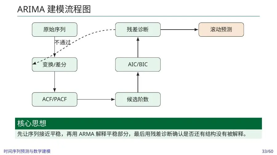
The I part stands for integrating after differencing. ARIMAmodels a series afterordinary differences if the raw level has a trend or unit-root-like behavior. With, the modeled quantity is roughly, and forecasts of differences must be accumulated back to the original sales level. If we difference a series that was already stable, we may add noise and make forecasts worse. If weekly seasonality remains, ordinary differencing may not remove it; a seasonal differenceor a calendar term may be more appropriate. The notation encodes what transformed series and lags are being used; it does not tell us whether they are justified.

Start with a few small candidate orders rather than automatically searching a giant grid. Inspect raw and transformed plots, ACF and PACF, and residual behavior. AIC or BIC penalizes extra parameters while rewarding fit within the modeled sample; rolling future performance is still needed. Suppose ARIMA(1,1,1) has lower AIC than ARIMA(0,1,1), but neither beats last-same-weekday forecasts on later Saturdays. The ranking among ARIMA candidates is not evidence that ARIMA supports the shop’s operational decision. It may be missing seasonality or promotions, or the simple baseline may genuinely be sufficient.

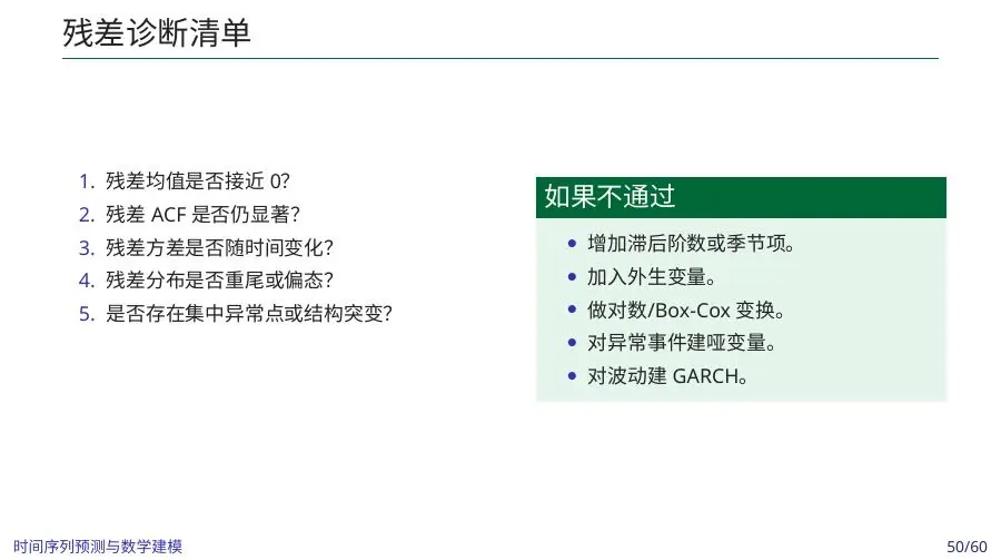
Residual diagnosis is a second mechanism test. After fitting, graph residuals by time, weekday, and promotion status; examine ACF and perhaps a Ljung–Box test for remaining serial correlation. If residuals repeat a weekly pattern, the model left predictable structure. If residual magnitude grows during high-volume periods, uncertainty may be level-dependent. If a model has tiny in-sample residuals but errors increase at rolling forecast origins, it may have overfit or relied on a regime that changed. Diagnostics and held-out errors ask different questions and should both be shown.

Seasonal ordersadd seasonal versions of AR, differencing, and MA. For monthly data with annual repetition,; for daily data with weekly repetition,; for hourly load with daily repetition,, although weekly structure may also matter. Multiple seasonality can exceed a simple single-season SARIMA configuration. SARIMAX includes external variables such as promotion, weather forecast, or planned price. At every rolling origin, those future covariates must be known or predicted separately. Feeding tomorrow’s observed weather into a historical SARIMAX test is not a valid forecast evaluation.

A minimal ARIMA fit looks like this:

from statsmodels.tsa.arima.model import ARIMA

model = ARIMA(train, order=(1, 1, 1))
fit = model.fit()
forecast = fit.get_forecast(steps=len(test))
mean = forecast.predicted_mean
interval = forecast.conf_int(alpha=0.05)

This code is not a model-selection procedure. Inspect the original series, justify differencing, compare several small orders using rolling validation, diagnose residual autocorrelation, and compare against naive and seasonal-naive forecasts.

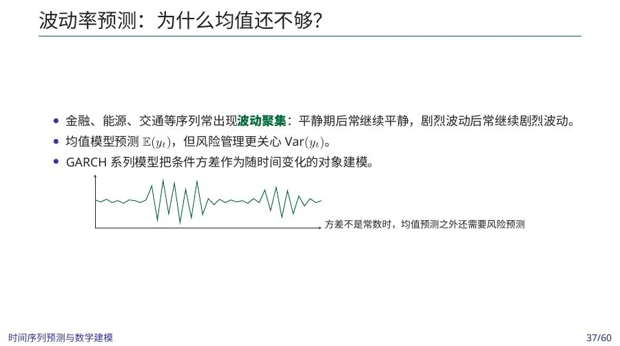
A forecast of the expected value is not always enough. In a financial or operational series, the size of surprises can change over time; volatility models try to forecast that changing uncertainty rather than just the level.

Difference for a reason, inspect ACF/PACF, compare small candidate orders, then test residuals and future weeks.

Volatility models

Financial returns may have weak mean predictability but clustered variance. A GARCHmodel uses

Its target is conditional volatility, not price direction. Verify that variance persistence and residual diagnostics support the model.

Forecast the size of shocks, not only their direction

Imagine a financial return series with many quiet days followed by several turbulent days. Its mean return may hover near zero throughout, but the magnitude of residuals changes. A constant-variance forecast interval built from all historical days can be too wide during quiet weeks and too narrow during turbulent weeks. An ARCH or GARCH model describes conditional variance as an evolving state informed by past squared surprises and past variance. It answers “how uncertain might tomorrow be?” rather than “will the price rise?” A modeler who interprets a GARCH volatility rise as a positive expected return has confused risk with direction.

Use the GARCH(1,1) equation above as an accounting update. Let,,in arbitrary consistent variance units for illustration. If previous squared shock was 4 and previous conditional variance was 1, the next variance forecast is. If previous shock were zero with same variance, it would be. The large surprise raises the next risk estimate even if its sign was negative; squaring removes direction. This is the intuition behind clustered volatility. Parameters must be constrained so variance remains nonnegative, and high persistencenear one means turbulence decays slowly. Numerical values here are illustrative, not a calibrated market model.

Volatility clustering can appear in nonfinancial operations too. Demand errors may be small most weeks but large during event-heavy periods. However a GARCH label is not automatically appropriate for lunch-box count errors. First check whether residual magnitudes remain serially dependent after trend, calendar, and known events are modeled, and whether the resulting risk forecast helps the actual inventory decision. If promotions are announced, a promotion-specific error range may be easier to explain and more useful than a generic variance recursion. Use the model that captures the supported uncertainty mechanism.

For an investment decision, connect mean and variance forecasts carefully. A mean model could forecast expected return, while a GARCH model forecasts conditional volatility of its residual or return. A portfolio also needs cross-asset covariance, transaction costs, and limits; one asset’s GARCH variance is not a complete risk model for a multi-asset allocation. Backtest any strategy at realistic rolling origins with costs and uncertainty. A lower price RMSE or a convincing volatility plot does not prove a better portfolio. The lecture’s risk slide is a reminder to evaluate the decision consequence of a forecast, not just the statistical fit.

Large residuals can follow large residuals even when average direction is hard to predict.

How long can a shock echo?

In the illustrative GARCH recursion,. A large squared shock raises today’s conditional variance through theterm, and tomorrow’s elevated variance feeds forward through theterm. The sum near one indicates persistence under standard model conditions: risk estimates can remain high for a while after turbulence. If the sum were much smaller, they would relax more quickly toward a background level. This is not a claim that market risk is controlled by a single number in reality; it is a parameter interpretation we must test against later residual magnitudes.

For the restaurant, suppose a week of promotion uncertainty creates errors of 30, 40, and 25 boxes after a long run of errors under ten. A constant error band from quiet weeks would be too narrow that week. Yet the cause may be the known promotion campaign, not an unexplained volatility process. A calendar-specific interval or scenario could be a stronger first model. If large errors still cluster after promotions, holidays, trend, and stockouts are accounted for, a conditional-variance model becomes a plausible candidate. The source of volatility should be diagnosed before a GARCH recursion is assigned to it.

The decision implication is a reserve, not a magical direction forecast. A busy-risk week might justify more ingredient safety stock or a flexible worker schedule, while a financial risk forecast could influence exposure limits under a separately defined policy. Measure whether the interval or reserve policy actually improves held-out cost and coverage. If a conditional-variance model predicts more risk but the realized distribution has much heavier tails than assumed, its nominal 95% interval may still under-cover. Residual magnitude and interval coverage are both necessary checks.

Grey forecasting

GMis designed for small, smooth, approximately exponential sequences. After accumulated generation,

it fits a first-order whitening equation. The accumulation suppresses noise but also imposes strong structure. Use it as a compact baseline for short, monotone series—not as a default for seasonal or highly volatile data.

What accumulated generation buys—and costs

Grey GM(1,1) is often introduced to students as a method that “works with few data points.” That is too generous unless we name its shape assumptions. Start with a short positive sequence. Accumulated generation forms running sums. For illustrative original values 2, 3, 4, and 5, accumulated values are 2, 5, 9, and 14. The running sum is smoother and always nondecreasing for positive inputs, even if individual values fluctuate slightly. GM(1,1) then fits a first-order response to that accumulated trajectory and inverse-accumulates predicted levels. It uses strong structure to compensate for sparse observations.

That strength is also its risk. A short seasonal series with values 2, 10, 2, 10 will still have a rising accumulated sum, but the original pattern alternates sharply; a smooth grey response can miss the next low or high. A sudden policy change can also be hidden by accumulation. If the original data are nearly monotone and approximately exponential over the required short horizon, a GM(1,1) trend may be a reasonable compact comparison. If the data show weekly or monthly seasonality, intermittent zeros, or unstable shocks, “small sample” is not evidence that grey prediction is appropriate. Test its level-ratio or admissibility conditions as taught in the deck, inspect original-scale residuals, and compare with a naive or simple trend baseline.

Think of a competition team with four annual production totals for a new service. There may be too little history to estimate a detailed seasonal model, and GM(1,1) might produce an easy-to-communicate short trend forecast. But the more honest forecast could be a scenario interval based on the service’s capacity and policy plans. A fitted curve through four points cannot identify every mechanism behind growth. Ask whether the downstream planning decision changes under a plausible slower-growth and faster-growth scenario. If the choice is stable, the exact grey forecast may not be crucial; if the choice changes, collect external evidence rather than quoting one deterministic GM(1,1) projection as certainty.

Grey modeling also teaches a lesson about transformations. The accumulated series is not the target the manager acts on; inverse accumulation must return forecasts to original annual or monthly units. Evaluate errors on the original series, not only on the smooth accumulated curve. Report how the tiny sample was selected and whether each historical point was available before the forecast date. A method with few fitted parameters can still be overconfident when the world changes after the observed window. Sparse data call for stronger assumption disclosure, not for a promise that one named technique solves uncertainty.

The GM(1,1) calculation behind the short name

The deck gives a concrete estimation recipe after accumulated generation. For each, construct a background value, the average of two adjacent accumulated levels. It approximates the accumulated state over that interval. Then fit the grey equation. Hereis the original increment from one accumulated value to the next;andare parameters. Put the observed increments in a vectorand rowsin a matrix, then estimateby least squares when the matrix is well-conditioned. With only a few data points, check sensitivity: a single revised observation can move the fitted parameters substantially.

For the toy sequence 2, 3, 4, 5, accumulated values are 2, 5, 9, 14. Background values forare 3.5, 7, and 11.5. The original increments to match are 3, 4, and 5. This little table tells us exactly what the grey fit is using. It does not just “fit a curve through four points”; it fits a relationship between the observed increment and a smoothed accumulated level. After estimating, the model predicts an accumulated response, and the original-scale forecast is the difference of successive predicted accumulated values. If we report the accumulated response itself as next year’s production, we have changed the target and overestimated its unit-scaled magnitude.

The differential-equation-like response under this fitted model iswhen. We need not memorize it to judge applicability. Ask whether the original levels are positive, reasonably smooth, and consistent with a short trend; check the deck’s level-ratio condition, residuals on the original scale, and comparison with a last-value or simple drift forecast. Ifis near zero, the expression’s separateterms can be numerically awkward even when a limiting trend interpretation exists. A computation that produces a precise-looking sequence from four observations is not automatically precise evidence about the future.

Suppose a competition question asks for production next year but a new policy may cap capacity. GM(1,1) trained on four years of growth may extrapolate through the cap because it has no policy variable. The correct forecast may be the minimum of an unconstrained demand scenario and a documented capacity scenario, or a model with explicit policy intervention. A model’s short name cannot replace an understanding of its data-generating assumptions. Grey prediction is useful when its strong short-trend assumption is plausible; it is dangerous when it becomes a ritual for every small dataset.

Regression and machine learning

Convert forecasting into supervised learning using lag features, rolling summaries, calendar indicators, and known external variables:

Tree ensembles capture nonlinear interactions. Neural sequence models may help with large, related datasets, but add tuning cost and leakage risks. Feature values must be available at forecast time.

A tree still needs to know which rows came before which

A supervised forecasting model turns each forecast origin into a feature row. For next Monday’s lunch-box demand, legal features might include last Monday’s sales, recent past weekday average, whether Monday is a holiday, and a promotion plan already announced by the order deadline. A tree model can capture nonlinear interactions, such as promotions mattering more on weekends, without a handwritten equation for every combination. But the tree has no built-in understanding of which dates are past or future. A rolling average calculated over a centered window, or tomorrow’s actual temperature slipped into its features, makes even a sophisticated model invalid for the operational question.

Suppose historical promotion days are rare. A tree can split sharply on the promotion flag and fit the few high sales exactly in training, yet its forecast for a new promotion may be unreliable. We need several later promotion events to evaluate that split; if none exist, show a wide scenario range. Similarly a model trained on observed sales during stockouts learns that high-demand days had low sales because inventory ran out. If the objective is true customer demand, sales are a censored observation: actual demand was at least sales, possibly more. Add stock-availability information and, where defensible, reconstruct or bound unmet demand. Otherwise the model may recommend too little inventory in precisely the weeks it sold out before.

An SVR or neural sequence model might fit richer patterns when many related series exist: dozens of stores, long histories, many known covariates. But more parameters bring tuning cost, data needs, and chances to exploit leakage. Compare them on exactly the same rolling origins and horizons as last-week-same-day, smoothing, and seasonal ARIMA. Include runtime and retraining burden if the owner must issue forecasts daily. If a neural model improves MAE by one box while being fragile on promotions and expensive to maintain, that one-box gain may not justify adoption. A model’s name is not an outcome.

External-variable forecasting has a hidden second forecast problem. If our model uses tomorrow’s temperature, we either need a weather forecast available now or must predict temperature ourselves. Its uncertainty should propagate into the lunch-box forecast or at least be tested through warm/cold scenarios. If it uses next month’s price, price must be a planned control or forecast; a future realized price cannot be treated as known. If it uses search activity at time, ask when that activity data are published and whether revisions occur. The feature availability ledger from the last lesson is the gatekeeper for every model class.

Cross-series learning also needs clean definitions. If one store measures orders placed and another measures lunches delivered, pooling them without harmonization can teach the model inconsistent targets. If a national holiday occurs on different dates or in different regions, one shared calendar flag may be wrong. Before asking whether a Transformer can learn dozens of sequences, ask whether those sequences count the same thing and whether their future information would be available at the same issue time. Model capacity cannot compensate for mismatched measurement contracts.

Compare methods from the same issue dates, with the same legal information and lead times.

Multi-step strategies

• recursive: predict one step and feed predictions forward;
• direct: fit a model for each horizon;
• multi-output: predict all horizons jointly.

Recursive forecasting accumulates error; direct forecasting uses fewer effective samples per horizon. Choose according to horizon and data volume.

A three-day forecast is not three one-day forecasts with hindsight

Suppose the restaurant orders ingredients on Sunday evening for Monday, Tuesday, and Wednesday. A one-day model can forecast Monday using Sunday’s known observations. But Tuesday’s forecast issued on Sunday cannot use actual Monday sales, because Monday has not happened yet. A recursive strategy predicts Monday, inserts that predicted value into the lag position that Monday would later occupy, then predicts Tuesday, and similarly for Wednesday. Errors in Monday’s estimate can feed into later estimates. If the model predicts 140 for Monday but actual Monday demand would be 180, the Tuesday forecast issued Sunday still has to work with its predicted 140, not the later observed 180. Using 180 in a historical Sunday-issued test is hindsight leakage.

A direct strategy fits a mapping for each lead time: Sunday features to Monday demand, Sunday features to Tuesday demand, and Sunday features to Wednesday demand. It avoids feeding one predicted target into the next, but each horizon-specific mapping has fewer effective training examples and may not share information as efficiently. A multi-output model predicts the whole three-day vector together, potentially learning that days within the order period move together. It may need more data and careful interval estimation. None is universally best; compare all plausible strategies at the same historical Sunday origins and assess day-one, day-two, and day-three errors separately.

Consider a strongly weekly restaurant. For next Monday, last Monday’s demand might be the most relevant naive forecast; for next Wednesday, last Wednesday’s might be. A recursive ARIMA model could still beat these if recent trend matters, but it must prove that on several later Sundays. If the business can top up ingredients Monday evening, the issue pattern changes: Tuesday’s operational forecast may then use Monday’s actual sales. A validation for a fixed three-day Sunday order cannot be copied as evidence for daily top-ups, and vice versa. The model strategy follows the purchase schedule.

The original-scale uncertainty also grows or changes by horizon. Monday might be fairly certain because a known office event is scheduled; Wednesday might be less certain because weather and event forecasts are farther out. A recursive model’s interval should account for uncertainty in its own fed-back predictions, not treat them as observed facts. Direct intervals should be calibrated separately at each horizon; a multi-output model may need to represent correlation across the days if the order quantity is total three-day ingredients. Reporting one grand MAE over all horizons hides where the approach fails.

For a longer three-month product-demand forecast, seasonality and external plans matter even more. Future promotions and prices may be known for month one but uncertain for months two and three. A model using those variables should either use a documented plan, forecast or scenario them, or exclude them at horizons where they are unavailable. If a method has excellent one-month performance but relies on a future price that the company cannot commit to, it may not be suitable for budget planning. Matching model inputs and strategy to horizon is part of comparing forecasts honestly.

Intervals and model risk

A point forecast hides uncertainty. Produce prediction intervals and check empirical coverage on rolling test windows. Intervals should account for observation noise, parameter uncertainty, and—when relevant—uncertain future regressors.

Compare models by horizon, season, and operating regime. A model may be best at one day and poor at one month. The final forecast model is the one that supports the downstream decision under realistic data availability, not the one with the most elaborate name.

The width of an interval is part of the answer

Suppose two models both forecast 140 boxes for tomorrow. Model A supplies a 90% prediction interval of 130 to 150; model B supplies 90 to 190. A manager facing costly stockouts may make different orders from these two results. The labels “90% interval” need validation: over many comparable historical issue dates, a calibrated interval should contain the realized demand about 90% of the time under the stated construction and conditions. One interval cannot verify its own coverage. A very wide interval can cover nearly everything but be too vague for staffing; a narrow one can look helpful while missing busy days too often. Report empirical coverage and width together, by horizon and regime.

What uncertainty goes inside? Observation noise—real day-to-day randomness—is one source. Fitted parameters are uncertain because history is finite. Future external predictors, such as weather or price, may also be uncertain. Structural breaks and stockouts can make old error patterns a poor guide to new conditions. Some analytic state-space forecasts propagate model-based uncertainty; bootstrap methods can resample suitable historical residual structure; quantile regression can predict lower and upper conditional outcomes directly. Whatever method is used, validate its intervals at rolling origins and show their failure cases. A closed-form 95% band from a misspecified model is not automatically a truthful 95% operational guarantee.

There is a common vocabulary trap: an interval for the estimated mean tomorrow is narrower than a prediction interval for tomorrow’s actual demand because the latter includes day-to-day variability. If the restaurant orders physical lunches, it cares about actual demand. A confidence band around an average seasonal effect is not a stockout-risk interval. Clearly label which quantity the interval covers. In financial returns, a volatility forecast likewise does not specify a complete extreme-loss probability unless a return distribution and tail behavior are assumed and checked.

Use a hand scenario before a statistical interval if data are sparse. Say ordinary weekday demand plausibly ranges from 120 to 150, while a known promotion could push it to 180. Ask how the order changes under each scenario and whether the promotion plan is confirmed. This does not create a formal probability, but it prevents the point forecast from hiding a decision-relevant uncertainty. Once enough held-out events exist, estimate and calibrate event-specific ranges. We can be more explicit with uncertainty without pretending the few available weeks justify a precise distribution.

Interval calibration can drift. If the shop expands seating or changes its opening hours, error distribution from earlier months may not apply. Monitor whether recent realized values fall below or above the interval more often than expected; inspect whether misses cluster by weekday or promotion. If the interval undercovers busy Saturdays, widen or remodel that regime, not necessarily every ordinary Tuesday. A model can remain good in mean prediction while its uncertainty estimate fails, and the inventory decision can fail because of that second error. Forecast maintenance is therefore not just retraining a point model; it is checking whether the stated uncertainty remains credible.

An interval is useful only when its coverage and width work for the decision.

Explain the choice as if a teammate has to run it tomorrow

Suppose the tournament finds that a seasonal-naive method has Monday MAE of 12 boxes, Holt–Winters has 11, and SARIMAX has 10 on the held-out Sundays. Which should the restaurant actually run? The answer is not automatically SARIMAX. Perhaps its two-box average edge comes mostly from one historical weather event and disappears when an archived weather forecast replaces the later observed temperature. Perhaps it gives much better calibrated high-demand intervals and lowers shortages enough to matter. Perhaps it fails when a promotion plan is missing, while the simpler methods remain available. The choice needs the error distribution, legal data inputs, decision cost, and failure behavior, not just a leaderboard.

An honest explanation could say: “For Monday–Wednesday orders issued Sunday evening, we selected seasonal-naive with an event-specific reserve because it matched the best complex candidate’s realized cost within uncertainty and used no future weather covariates. It underpredicted after the spring menu change, so we now monitor four-week bias and will refit a level adjustment if the drift persists.” Or it could say: “We selected SARIMAX because the promotion plans are fixed before Sunday, its intervals covered held-out promoted days more reliably, and that reduced expensive shortages; when the promotion feed is stale, the system falls back to last-same-weekday.” Each explanation tells the next teammate what to run, what data they need, and when not to trust it.

The fitted order or algorithm settings should be reproducible: training interval, transformations, candidate orders or smoothing settings, event definitions, issue-time covariate sources, historical origins, horizon, and error metric. This is documentation of a decision, not a ceremonial table. If a new analyst cannot reconstruct one historical Sunday forecast from the description, claims about rolling performance are difficult to audit. Record the version and data snapshot for each issued forecast, especially when source files are later corrected. A model choice is strongest when it survives an independent rerun.

Be transparent about uncertainty in the comparison itself. If we tested only four Sundays, an apparent one-box MAE difference could be chance. A model that narrowly wins in one semester may fail after a new café opens. Show performance across many origins when possible and inspect whether the winner changes by holiday or season. If two methods are practically tied, the one with simpler inputs or better failure handling may be preferable. The goal is a defensible forecasting workflow, not a trophy for one model name.

We have several candidate models, and their names alone do not tell us which helps the decision. We will give each the same historical information and evaluate them on the same future periods, including a plain baseline.

Compare forecasts fairly

Use monthly product demand as a running example. The series has five years of history, annual seasonality, promotions, and occasional stockouts. The business needs forecasts for the next three months. A model tournament compares candidates under exactly this information pattern.

Start with baselines

Define naive, seasonal-naive, mean, drift, and moving-average forecasts. The seasonal-naive forecastis often difficult to beat for strongly seasonal monthly data. If a sophisticated model wins only against the mean, the comparison is incomplete.

One fair Sunday-origin tournament

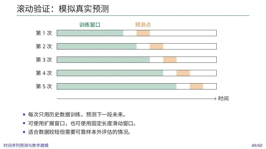
Let us choose a concrete operating pattern: every Sunday evening, the restaurant orders ingredients for Monday through Wednesday. We have a year of daily box sales, documented closure days and promotions, and archived weather forecasts as issued on past Sundays. The first historical origin might be a Sunday after three months of training. At that origin, each candidate gets the same past sales, the same known calendar, and the same weather forecast. It produces three forecasts and, if it claims them, three intervals. Then we advance to the next Sunday, refit or update each candidate as its procedure requires, and repeat. This is a tournament because methods face the same future days under the same information, not because we try to crown the most complex algorithm.

Compare last-same-weekday, a trailing weighted average, Holt–Winters if there is stable weekly seasonality, a small SARIMA or SARIMAX candidate, and perhaps a tree with lag/calendar features. A single promoted Saturday in training cannot teach all models a reliable promotion effect; if the manager’s Monday–Wednesday orders do not include promotions, focus first on ordinary operating days and stress-test special events separately. If a candidate uses a future regressor, confirm it was actually known at each Sunday origin. A retrospective actual weather measurement must not replace the archived Sunday forecast for Tuesday.

Store each origin’s predictions rather than only printing one aggregate number. For Monday, Tuesday, and Wednesday separately, calculate MAE, bias, RMSE if large misses matter, and empirical interval coverage. Plot errors over calendar time: a model can win on average yet fail after a menu change. Label underpredictions and overpredictions separately. If last-same-weekday has MAE 12 boxes and SARIMAX has MAE 10 but systematically underpredicts hot days, a two-box average advantage might not settle the ingredient order. Test the order rule and cost on both models’ forecasts.

Runtime and maintainability count as operational outcomes. If a complex model needs several hours of tuning or fails to converge on one Sunday, the manager needs a fallback. State what the fallback is—perhaps last-same-weekday plus a tested reserve—and when it will be invoked. An honest benchmark report can select a simple method if no more complex candidate offers a meaningful improvement. That is not a failure to use mathematics; the rolling comparison itself is the evidence supporting the choice.

Finally keep a late untouched test period after choosing the workflow. Repeatedly editing the model after seeing that final period makes it another validation set. If the test result is disappointing, report it and explain what changed, then collect or reserve a later period for the revised method. A lesson that only displays the victorious training-period curve would teach students how to overfit, not how to forecast. Historical issue times and a fair baseline are the backbone of the whole comparison.

Understand exponential smoothing

Simple exponential smoothing updates level:

near one reacts quickly; near zero smooths strongly. Holt adds trend; damped Holt prevents indefinite linear growth; Holt–Winters adds seasonality. Estimate smoothing parameters by minimizing one-step errors or likelihood rather than choosing them from visual smoothness.

Read ARIMA notation

ARIMAappliesdifferences and models the remainder withautoregressive lags andlagged shocks. SARIMA adds seasonal orders. ACF/PACF patterns can suggest orders, but information criteria and rolling validation decide among plausible candidates. After fitting, residuals should have near-zero mean, stable variance, and no material autocorrelation; a Ljung–Box test supports but does not replace the residual plots.

Treat interventions and external variables honestly

Promotion, price, weather, and holidays can enter dynamic regression. Future values must be known or separately forecast. Stockouts censor demand: observed sales are less than latent demand, so a model trained on sales may learn artificial low demand. Add availability indicators, reconstruct censored demand when defensible, or state the limitation.

Structural breaks require intervention variables, shorter training windows, time-varying parameters, or regime models. Do not hide a pandemic or policy change inside a generic outlier-cleaning rule.

Generate intervals

Intervals should widen with horizon. Analytic state-space models can propagate uncertainty; bootstrap methods resample suitable residual blocks; quantile regression directly predicts conditional quantiles. Evaluate empirical coverage and average width together. A 95% interval that covers 100% because it is enormous is not automatically useful.

Compare over rolling origins

For each origin, fit using only available history and forecast horizons 1–3. Store every prediction, not only aggregate scores. Report MAE, RMSE, MASE, bias, and interval coverage by horizon. Use a loss function aligned with decisions: underprediction may be more costly than overprediction in capacity planning.

from statsmodels.tsa.statespace.sarimax import SARIMAX

model = SARIMAX(
    train,
    order=(1, 1, 1),
    seasonal_order=(1, 1, 1, 12),
    enforce_stationarity=False,
)
fit = model.fit(disp=False)
forecast = fit.get_forecast(steps=3)
mean = forecast.predicted_mean
interval = forecast.conf_int(alpha=0.05)

This code is a candidate, not a conclusion. The final selection table must compare it with baselines and alternatives over all origins.

One month-end forecast you can audit

Return to the beverage company’s monthly demand. Assume last January, February, and March sold 800, 850, and 900 units, while this January, February, and March sold 880, 920, and 980. At the end of this March, a seasonal-naive forecast for coming April would use last April’s demand, which we have not listed; a model that reports a numerical April forecast without that value is inventing an input. Suppose last April actually sold 950 units. Then seasonal-naive April forecast is 950. A simple “last observed month” baseline gives 980, but it ignores the usual March-to-April seasonal shift. The two forecasts answer different assumptions: repeat annual position or repeat current level. We can compare them on many earlier month-end origins rather than declaring one right from this single April.

Imagine the company has already announced an April promotion. If historical April 950 had no promotion and the new one does, a SARIMAX or regression approach could adjust for the planned event, but only if several earlier comparable promotions support an effect. We cannot borrow a “promotion uplift” from future actual April sales and claim it was known in March. A decision report might present 950 as the seasonal baseline, a supported promotion scenario of perhaps 1,050, and a stress outcome of 1,200 with clearly stated assumptions. Those scenario values are illustrative, not an estimated company forecast. Production should then be tested under storage, overtime, and shortage costs.

The audit trail for this one forecast is short enough to inspect. We need the issue date at March close; last April’s 950; the announced April promotion plan and its date; any weather or price forecast that existed by issue time; the exact method version; the issued point or interval; and actual April demand after the month ends. If the model uses revised March sales that were not finalized until mid-April, the historical test is unfair. If it uses only observed sales but April stocked out, actual April sales are a lower bound on demand. If the promotion is cancelled after issue, that is a changed input scenario, not evidence the forecast code was numerically wrong.

This compact case shows how model comparison should feel to a new analyst: take one origin, list the legal inputs, hand-calculate a baseline, run each candidate, and follow the output to a production action. Then repeat on many origins. There is no virtue in a large leaderboard whose rows cannot be traced to one real historical decision. The strongest forecasting section lets a skeptical teammate pick any date and reproduce both the prediction and the reason for trusting or distrusting it.

Model map from the full lecture

Exponential smoothing family

Simple exponential smoothing handles a changing level. Holt adds trend; damped Holt prevents indefinite linear growth; Holt–Winters adds additive or multiplicative seasonality. Additive seasonality has roughly constant amplitude; multiplicative seasonality scales with level. State-space implementations provide likelihood-based estimation and intervals.

ARIMA and SARIMAX

ARIMAmodels differenced history with autoregressive and moving-average terms. Seasonal ARIMA adds. SARIMAX includes external predictors, but future values of those predictors must actually be known or separately forecast. Select a small candidate set using ACF/PACF and AIC/BIC, then decide with rolling performance and residual white-noise checks.

A monthly seasonal model with a promotion plan

Suppose a beverage company has five years of monthly demand and wants to decide the next three months’ production. Sales rise each summer, drift upward slowly over years, and spike during scheduled promotions. A seasonal-naive forecast for each future month repeats the same month last year. This is a strong baseline because it captures summer timing without fitting many parameters. If last July sold 1,000 units and this July’s promotion is similar, predicting about 1,000 is not foolish merely because it uses a single historical value. The baseline becomes weaker if the whole market has grown or a new promotion differs. That is where Holt–Winters, SARIMA, or SARIMAX might add value.

SARIMA notationuses ordinary and annual-seasonal lag structures. A seasonal difference compares each month with the same month a year earlier. If July demand rose from 1,000 to 1,100 across years, the difference is 100 units; modeling those changes can help adapt to a trend. But if a one-time promotion raised one July to 1,500, the seasonal difference can carry that shock into next July’s comparison. Include a documented promotion variable or intervention rather than forcing seasonal coefficients to explain a special event. The model order chosen from ACF, PACF, or AIC is a candidate description of historical dependence; future validation decides whether it outperforms the seasonal-naive baseline.

With SARIMAX, a future promotion flag can enter if the company has already set the campaign calendar at the forecast issue date. A planned discount or price may also be known if management has committed to it. If the campaign is still under discussion, run scenarios: no promotion, modest promotion, and strong promotion with supported effect ranges. Do not take the actual future promotional spend from a historical dataset and pretend it was known three months in advance at each rolling origin. This is why archived plans or issue-time snapshots can matter as much as the sales table. Forecasting an external variable separately can compound uncertainty; report that extra assumption.

Stockouts create a further issue. If July demand could have been 1,300 but warehouse stock was only 1,100, observed sales of 1,100 are a lower bound on demand, not a true demand measure. A model trained on sales may infer demand plateaued and underproduce next year. Inventory records and lost-order logs can help reconstruct or bound latent demand. If they do not exist, state that the model forecasts observed sales under prior stock policy, not unconstrained customer interest. Using a sophisticated SARIMAX implementation on a censored target cannot repair the target definition.

At each historical month-end origin, compare three-month forecasts from seasonal-naive, an appropriate smoothing model, and a small seasonal ARIMA or SARIMAX candidate using only plans known then. Report horizon-one, horizon-two, and horizon-three errors and interval coverage. Then apply forecasts to production constraints: overtime, storage, unmet orders, and promotional commitments. If seasonal-naive wins most ordinary months while SARIMAX helps only planned promotions, a hybrid or scenario-based approach may be more maintainable than one complex model used everywhere. The decision is not “which method has the cleverest notation?” but “which workflow supports reliable production under the information pattern we actually have?”

ARCH/GARCH

When residual magnitude clusters, model conditional variance:

GARCH answers risk and interval questions that a mean forecast misses. Check positivity and persistence; values near one imply slow volatility decay.

Grey, Markov, and VAR models

GM(1,1) is designed for very short, smooth positive series: accumulate data, fit a first-order response, and inverse-accumulate predictions. Test level-ratio conditions and compare with naive forecasts; small sample size is not evidence of validity.

A Markov chain models discrete state transitions. It is useful for regimes, ratings, or weather states when the state definition is meaningful. VAR models multiple endogenous series,

and supports impulse responses, but parameter count grows asand stationarity/cointegration must be addressed.

A state forecast when a number is not the natural output

Sometimes the decision is not “how many boxes?” but “will tomorrow be a quiet, ordinary, or busy day?” Define states with operational meaning, perhaps quiet below 110 boxes, ordinary from 110 to 160, and busy above 160. A Markov model estimates how often each state follows another. If historical quiet days were followed by ordinary days 60% of the time and quiet days 40% of the time, that row of a transition matrix gives a simple next-state forecast. Every row must sum to one; a negative transition probability or a row totaling 1.3 is invalid. The thresholds should be chosen for a business decision, not simply to make three equal-sized bins.

The Markov assumption says next state’s distribution depends on the current state under the specified model, not the entire prior history. A shop whose busy days follow scheduled promotions may violate that if promotion plans are not included. A summer busy day and a winter busy day may also have different next-day behavior. Estimate transitions within training history and validate on later weeks; if the matrix changes by season or policy, report that instead of treating one global matrix as a law. A state model can be intuitive for shift planning when staffing comes in discrete levels, but it may throw away within-state magnitude needed for ingredient orders. Choose it when state transitions match the decision.

VAR asks a different question: can several time series help predict one another? Suppose lunch-box demand, beverage demand, and foot traffic move together. A vector autoregression uses their lagged values to forecast the vector jointly. Withseries andlags, coefficient count grows roughly likebefore constants and extra terms; even a moderate set of related series can outrun a short history. Check whether all series have consistent timestamps and whether their transformed behavior fits the assumptions. A foot-traffic series recorded after closing cannot help a morning forecast of the same day without leakage.

Impulse responses in VAR can describe how a modeled shock in one series is followed by changes in others, but interpretation depends on assumptions about shock identification and the fitted system. If a beverage promotion raises both drinks and lunches, a VAR correlation might reflect the shared promotion rather than beverage sales causing lunch sales. For a beginner course, the safest reading is “these observed series contain lagged predictive information under this model,” not a causal claim. If the decision needs a causal effect of a promotion, design, timing, and external variables deserve separate treatment.

Grey forecasting, Markov states, and VAR thus answer different kinds of questions. Grey forecasting compresses a short smooth trend. Markov models transition between meaningful discrete regimes. VAR uses interactions among several measured histories. We do not select among them by a ranking of fashionable method names. We inspect data volume, variable definitions, horizons, forecast-time availability, and held-out decision performance. A simple seasonal-naive forecast may still beat all three for a weekly shop even though their mathematics is richer.

Regression, trees, and neural models

Supervised models need lag features, rolling statistics, calendar variables, and known external factors. Trees capture nonlinear interactions; SVR works on medium data; neural sequence models demand more data and stronger baselines. Fit feature transformations inside each rolling fold. Direct multi-horizon models avoid recursive error accumulation; recursive models are cheaper; multi-output models exploit cross-horizon structure.

The model map separated methods by the kind of pattern they address. Two complete cases now show how an analyst moves from a forecast score to a real choice—and how a seemingly small error can matter differently in different decisions.

The output of a forecast is an action under uncertainty, followed by a check against the realized outcome.

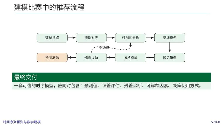
A clinic queue tests what the model selection really means

The lecture lists hospital visits among time-series examples. Suppose a clinic must schedule nurses for next week’s daily visits. A seasonal-naive forecast repeats last week’s same weekday visits. A Holt–Winters model may adapt to changing level and stable weekday patterns. A regression model may include known public holidays and planned clinic hours. A SARIMAX candidate may model lagged residual dependence plus those external factors. The clinic’s decision is not simply average visits: an understaffed busy day can create long waits, while extra nurses are costly. The relevant horizon is next week as of the shift-schedule deadline, not a one-day forecast updated after each day begins.

Suppose Monday visits in four recent weeks were 80, 82, 85, and 120; the fourth Monday included an unusual vaccination event. A naive last-Monday forecast of 120 for next ordinary Monday might overstaff, while a smoothed level around 90 might be better. But if next Monday has another planned campaign, the last event may be relevant. The question cannot be settled by clipping 120 as an outlier. We need the event calendar and its publication time. A model that uses a flag for next Monday’s campaign is valid only if the campaign was known when the roster was set. A fitted “event effect” from one past campaign is uncertain; present a scenario range rather than a sharp coefficient.

Clinic visits may also have day-of-week seasonality and longer winter peaks. A 168-hour ACF in hourly visit arrivals could reveal weekly recurrence, but a daily staffing plan may only need weekday counts and peak-hour arrivals. Aggregating visits to a daily total can hide a noon rush where queue service breaks down. If staffing is hourly, evaluate hourly forecasts and queue consequences; if staffing is daily, explain why daily counts suffice or add a stress test for peak hours. Model frequency follows the decision. This is the same lesson learned from transformer load and lunch-box ingredients, applied to people waiting for care.

At each historical roster date, compare forecasts from seasonal-naive, smoothing, and one more complex candidate, then convert each to a shift plan using the same staffing rule. Score realized overtime, wait-time proxies, and unnecessary staffing under stated assumptions, alongside MAE and interval coverage. A candidate may reduce overall count error but miss the specific days that breach a queue threshold. If so, inspect its busy-day tail and calendar variables. It might need a better interval, a structural event model, or a conservative reserve—not necessarily a deeper neural network. A forecast model earns its place by improving the clinic’s action under realistic uncertainty.

This case is not a clinical staffing recommendation. The visit counts and costs are illustrative, and patient-care standards require real evidence and professional oversight. In a student modeling lesson, it demonstrates how to trace a technical metric to an operational threshold and how to declare a limitation. A paper that reports one model’s lowest RMSE while ignoring known campaigns and waiting times has not yet answered the clinic’s question.

Two complete decision cases

For sales-to-inventory, forecast demand distribution, not just the mean. If ordering, demand, holding cost, and shortage cost, the forecast enters

Evaluate final inventory cost as well as MAE. For investment series, forecast expected return and conditional covariance, then feed both into a mean–variance or robust allocation. Backtest with transaction costs and rolling re-estimation; a lower price RMSE does not guarantee a better portfolio.

Lunches: choose an order from a distribution

The inventory expression above can be read as a balance between leftovers and unmet demand. If the restaurant ordersboxes and actual demand is, leftover count isand shortage count is. Let illustrative leftover cost be8 per box. For a toy demand distribution with three equally likely outcomes 110, 140, and 180 boxes, ordering 140 creates costs0, and136.67. Ordering 180 creates leftover costs120, and110. Ordering 110 creates shortages240, and266.67. Among these three candidate orders, 180 has the lowest expected illustrative penalty despite 140 being the middle demand value.

These costs are invented, and “equal likelihood” is a pedagogical assumption rather than a calibrated forecast. A real order also pays ingredient cost, earns sales contribution, faces preparation capacity, and may salvage leftovers. Once those quantities are known, revise the objective. The hand calculation’s purpose is to show why point MAE and best inventory choice need not rank models the same way. If shortages cost far more than leftovers, an upper demand quantile can be more useful than the mean. If leftovers are expensive, the balance changes. Forecasting and optimization are two stages of one decision pipeline.

Now compare forecast methods by realized costs across historical Sundays: at each origin, use the method’s predicted distribution or scenarios to choose a Monday order, then score it against actual Monday demand under the same cost rule. One model may have slightly worse point MAE but better-calibrated busy-day tails and lower cost. Conversely a model can report attractive wide intervals and still make expensive overorders. The tournament should show both statistical metrics and decision outcomes. This is what the lecture means when it says forecasting is often an intermediate modeling step.

Investment: a risk forecast is not a buy signal

For an investment series, predicting average return and forecasting volatility address different aspects of allocation. A GARCH variance estimate can rise after turbulent returns while expected return remains near zero. If a team sends both to a mean–variance portfolio optimizer, it also needs how assets co-move, constraints on holdings, transaction costs, and the investor’s risk tolerance. A one-asset conditional variance is not a full covariance matrix. A backtest must use only prices and estimates known before each trade, include turnover costs, and compare with a plain benchmark portfolio. An attractive in-sample return curve with later prices leaking into fitted forecasts is not evidence of a strategy.

Suppose one candidate forecasts prices with low RMSE but always lags large reversals; another has higher price RMSE but signals lower risk before volatile periods. Neither automatically wins an allocation comparison. The actual evaluation may be drawdown, risk-adjusted return, turnover, or probability of breaching a risk limit. State the objective before model selection. For a beginner, a simple no-trade or balanced portfolio benchmark can be illuminating: if predictive complexity does not improve a cost-aware rolling backtest, it may not justify taking on trading risk. The course’s modeling principle travels from lunch boxes to finance, even though their loss functions and constraints differ.

Know the data, beat a baseline, validate in time order, and connect predictions to actions.

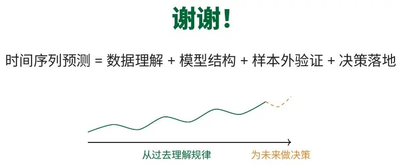
A forecast workflow needs a failure signal

Imagine the restaurant’s selected seasonal-naive-plus-reserve method worked well during autumn, but a new office opens nearby in spring. For several weeks the method underpredicts Monday through Wednesday by about 30 boxes. If we keep reporting its old autumn MAE, we are describing a history that no longer matches current demand. Monitor rolling bias and error by weekday, interval coverage, and downstream shortages. A persistent positive actual-minus-forecast residual is a signal to update level or investigate the new source of customers. One unusually busy day is not enough to refit everything; a repeated pattern is stronger evidence of a regime shift.

Suppose a forecasting system uses yesterday’s sales as a feature and the register stops uploading at the end of each day. The model may still run by filling yesterday with a default, but its legal input contract has failed. A production workflow should alert on stale data, impossible values, missing promotions, or unissued weather forecasts and switch to a documented baseline when necessary. “Model converged” is not the same as “forecast used valid current inputs.” A simple fallback tested historically is more useful than a complex method that quietly continues after its key covariate disappears.

Retraining can also erase useful history if done blindly. If the menu changes permanently, a recent sliding window may adapt faster than an expanding window including old menu demand. If a temporary festival caused one busy week, throwing out all old weeks may overreact. Try both strategies on later origins and keep event annotations. Forecast monitoring is an ongoing comparison between mechanism, data definition, and decision loss. If decision costs or capacity change, re-evaluate methods even when point MAE stays similar: a new shortage penalty can change which forecast distribution is most useful.

Intervals must be monitored separately from means. A forecast may retain zero average bias but have much larger errors during holiday seasons, causing a 90% interval to cover only 60% of realized holiday days. The fix may be regime-specific uncertainty, better event predictors, or wider stress scenarios; simply moving the point forecast up will not solve symmetric uncertainty growth. Report recent coverage and width by horizon, not only an overall number blended with quiet months. The manager needs to know whether “140 plus or minus ten” still has evidence behind it.

Finally preserve a model-decision log. For each issue date, record data available, candidate versions, issued forecast and interval, chosen order or allocation, and realized outcome when it arrives. This supports a genuinely fair backtest and makes failures diagnosable. If the team retrospectively reconstructs forecasts from a current spreadsheet that has been corrected and revised, it may accidentally use information not available on the original date. A modest archive of issue-time snapshots is part of reliable modeling. The most valuable mathematical model is one whose forecast, uncertainty, and decision can be audited after the world has moved on.

Tell the forecast story in a modeling paper

The deck also asks how a forecasting method belongs in a mathematical-modeling paper. Begin with the decision and horizon: “We need next-week demand issued every Sunday to set ingredient orders.” Then define the observed target, calendar frequency, closure and stockout rules, and which future covariates are genuinely known by Sunday. Show a raw time plot annotated with promotions and breaks before displaying model notation. A reader should understand why a weekly seasonal baseline is natural and why a promotion variable is even available. If the paper starts with “we fitted ARIMA(2,1,3)” but never defines the issue time or demand measure, it has hidden the most consequential assumptions.

After the data story, show the comparison fairly. State the training history, rolling origins, three-day lead times, baselines, and selection metric; report errors and coverage by day rather than only one average. Explain whether differencing, log transformation, or seasonal terms were used and how outputs return to units of lunches. Include one residual or failure-pattern plot: weekly structure left behind, promo errors, a new level after a menu change, or interval misses on busy days. A small honest candidate set is more persuasive than an unreported grid search that quietly tried hundreds of combinations until one won on the test month.

Then move from forecast to action. For the restaurant, convert each candidate’s forecast or demand scenarios into an order under stated leftover and shortage costs. Show one hand calculation like the 110/140/180 scenario above, with units and clearly illustrative prices, then score decisions over later Sundays. State what happens when a promotion plan or weather forecast is unavailable; a baseline fallback should be in the paper because that is how the system works on bad-data days. If the forecast interval does not cover enough held-out outcomes, say so before using it to justify a reserve.

Close with a boundary, not a victory claim. Perhaps the chosen workflow performed well on ordinary school-term weekdays but had only two documented promotions, so promotion uncertainty remains wide. Perhaps a stockout means observed sales did not reveal true demand. Perhaps next year’s market size could change. A conclusion can recommend a near-term operational method and a monitoring trigger while acknowledging those limits. In a modeling competition, that clarity usually makes the mathematics feel more reliable, not less. The strongest paper lets another team reconstruct one forecast and one decision from the available information at its issue date.

This writing order is also a teaching order. We met the last-value and seasonal-naive methods first because they expose assumptions in plain language. Smoothing adds adaptive level, ARIMA adds lag and shock structure, SARIMAX adds known outside influences, GARCH addresses changing risk, grey modeling compresses sparse smooth trends, and trees or neural methods add flexible interactions when data support them. The methods are tools for distinct patterns; the question, data clock, baseline, uncertainty, and action remain the spine of the story.

Here is a useful final counterexample. Suppose a deep sequence model forecasts tomorrow’s lunches with MAE 8 boxes on a randomly shuffled test split, while last-same-weekday has MAE 12. When we rerun at real Sunday origins, the deep model’s MAE rises to 18 because its centered rolling features had included later demand and because March’s menu-change days were spread into training and test. Last-same-weekday remains at 12. The correct response is not to declare all neural forecasting useless; it is to repair feature timing, separate the regime change, retrain within each historical origin, and then compare again. If the repaired deep method still wins, use it with a documented data and failure contract. If it does not, the earlier six-box “gain” was a validation artifact.

The same logic catches a seasonal model whose intervals are too narrow. Suppose SARIMA’s point MAE is ten, matching the best alternative, but its nominal 90% interval covers only six of ten later promoted days. Ten events are still few, yet the miss pattern is enough to question whether promotion uncertainty is represented. We might show wider scenarios for promotions, collect more campaign history, or avoid sharp claims for those dates. A model can be successful on ordinary days and uncertain on special ones; that qualified conclusion is more useful than one global accuracy adjective.

All numerical examples in this lesson—the lunch-box counts, monthly beverage totals, toy GARCH parameters, clinic arrivals, and three-demand inventory outcomes—are instructional inventions. The model families, workflows, and figures are drawn from the course deck, while technical implementation links point to official library documentation. Reuse the derivation and validation discipline; replace every toy number with real source evidence before acting. A beginner who remembers only one rule should remember to hand-calculate an honest baseline at one issue date, then require every more advanced method to forecast under that same information and earn a better decision.

There is no contradiction between choosing a very simple forecast for next week’s lunches and a more structured model for three-month production or risk. The horizons, series lengths, known future plans, and losses differ. The best method can also change after a menu redesign or stock policy shift, because the target and information process have changed. A course that teaches only equations would miss that practical fact. Forecasting is a repeated experiment at historical issue dates, followed by a decision whose costs reveal whether the experiment mattered. Keep the issue-time data, baseline, and realized outcomes together; they are what allow the next analyst to improve the method without reinventing its story.

A forecast is useful only if its horizon, uncertainty, and comparison match the decision. Before we trust more complex analysis, the next lesson returns to the raw observations and asks whether their rows, missing values, and units mean what we think they mean.