LLM 5 - Pretraining, Scaling, and Domain Models

Welcome back. In LLM 2 we opened the Transformer, and in LLM 3-4 we followed a pretrained model into prompting, tools, and retrieval. This blog moves in the opposite direction. Before a model can answer a prompt, where did its behavior come from? What exactly was optimized during pretraining? Why can a model fit for inference but run out of memory during training? When does adding GPUs help, and when does it merely duplicate the same memory problem? Finally, if the goal is financial language rather than general web text, should we train a specialist, adapt a general model, or mix both kinds of data from the beginning?

We can answer those questions by separating three layers that are easy to confuse:

1. The learning problem: choose an architecture, a tokenizer, a data distribution, and a self-supervised objective.
2. The systems problem: store weights, activations, gradients, and optimizer states while moving the right tensors between accelerators.
3. The allocation problem: under a fixed budget, decide how much compute belongs to model parameters and how much belongs to training tokens.

We will connect those layers rather than treating pretraining as one enormous call to train(). BloombergGPT will be our running case study near the end: not because every domain model should copy it, but because it makes the tradeoffs concrete.

Choose Before You Train

Start from the Product, Not the Parameter Count

A generative-AI project does not begin with “Which GPU should we rent?” It begins with a use case and an acceptance test. Do we need a classifier, a writing assistant, a private search interface, a code generator, or a model whose weights can run inside a controlled environment? The answer changes what kind of model is useful and whether pretraining is justified at all.

A useful project lifecycle is a sequence of decisions:

• Scope: define the use case, users, data boundary, latency target, failure cost, and evaluation set.
• Select: reuse an existing model or pretrain one.
• Adapt and align: prompt, retrieve, fine-tune, or use human feedback; then evaluate.
• Integrate: optimize inference, deploy, monitor, and connect the model to the application.

Model selection sits inside a larger lifecycle. Pretraining is one possible decision, not the automatic first step. Course slide 3.

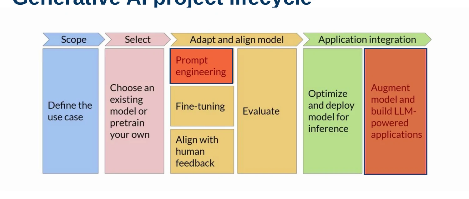
Notice the asymmetry: choosing to pretrain affects every later stage, but later evidence can force us to revisit the choice. If a retrieval system already meets the factuality target, pretraining a new model may add expense without solving the real bottleneck. If the vocabulary, language, licensing boundary, or domain distribution is fundamentally different from available models, custom pretraining may become defensible.

Reuse, Adapt, Continue, or Start from Scratch

There are four progressively more expensive options.

Use a pretrained model as-is. Prompting and retrieval leave its parameters unchanged. This is the fastest path when the base model already has the required language ability and the missing information can be supplied at inference time.

Fine-tune a pretrained model. Supervised fine-tuning or parameter-efficient methods modify behavior using task examples. Fine-tuning is appropriate when the model knows the underlying language but does not reliably follow the desired format, policy, style, or decision boundary.

Continue pretraining. Domain-adaptive pretraining resumes a self-supervised objective on domain text. It is useful when the model must internalize recurring terminology, syntax, or statistical structure that is poorly represented in the original corpus. Continued pretraining is not the same as teaching a task with labeled examples.

Pretrain from scratch. This gives maximum control over tokenizer, architecture, data mixture, and checkpoints, but it also requires the largest corpus, engineering effort, evaluation program, and compute budget. “We possess private documents” is not by itself a reason to do this; retrieval or continued pretraining may be enough.

Decision rule. Spend compute only on a limitation that measurement has identified. Prompting changes the current context, fine-tuning changes behavior, retrieval changes available evidence, continued pretraining changes the learned domain distribution, and pretraining from scratch changes the entire foundation.

Read a Model Card Before Downloading Weights

Model hubs make weights easy to find, but a repository name is not a deployment specification. A useful model card should tell us at least:

• architecture and parameter count;
• tokenizer and context length;
• training objective and data summary;
• license and restrictions;
• expected inputs and outputs;
• benchmark results and evaluation conditions;
• known limitations, biases, and intended uses;
• hardware or precision requirements.

The model with the largest benchmark number may be unusable under the target license, too slow for the latency budget, incompatible with the input language, or impossible to fit on the available hardware. Selection therefore combines quality, cost, governance, and operational constraints.

Pretraining Is Only One Stage

Pretraining learns broad statistical regularities from large unlabeled corpora. It does not automatically produce a safe assistant, a calibrated classifier, a citation system, or a domain-approved decision maker. Instruction tuning, preference optimization, retrieval, tool use, red-teaming, monitoring, and product controls address different layers.

This distinction matters when evaluating a failure. If the model does not recognize financial abbreviations, the representation or training distribution may be weak. If it knows the terms but ignores a requested JSON schema, instruction tuning or output validation may be weak. If it confidently reports yesterday’s price, the system may need current retrieval. Calling all three failures “the model needs more pretraining” wastes both time and compute.

Pretraining Objectives

Self-Supervision Creates Its Own Targets

Human labeling does not scale to trillions of tokens. Language-model pretraining instead derives a target from the text itself. A tokenizer maps documents into token IDs, an objective hides or shifts part of the sequence, and the model predicts the withheld information. The same document supplies both input and target.

Let a tokenized sequence be . A general pretraining loss is an average negative log-likelihood,

where is the set of prediction positions. The architecture and corruption rule determine visible and . That choice is not cosmetic: it determines what information each hidden state can use and what kind of behavior training directly rewards.

Encoder-Only: Masked Language Modeling

An autoencoding encoder such as BERT replaces selected input tokens with a mask or another corruption and reconstructs them from both left and right context. If position is selected,

where is the masked set and is the corrupted sequence. Bidirectional visibility makes these representations natural for sentiment analysis, named-entity recognition, token classification, and other tasks that inspect a complete input. BERT and RoBERTa are representative encoder-only models.

The limitation is equally important. The model is trained to fill selected holes, not to continue a sequence indefinitely from left to right. We can attach task heads to its contextual states, but it is not naturally a free-form generator.

Decoder-Only: Causal Language Modeling

An autoregressive decoder predicts the next token using only its prefix:

A causal attention mask blocks future positions. Because generation repeats exactly this operation—predict, append, predict again—the objective aligns naturally with text and code generation. GPT, BLOOM, and BloombergGPT are decoder-only examples. Abilities that look like classification, question answering, or tool selection can also be expressed as continuation tasks when the model and prompt are sufficiently capable.

“Autoregressive” does not mean the model has access to only one previous token. It may attend to the entire available prefix. “Unidirectional” describes the information boundary at each prediction position, not the number of layers or the richness of the context.

Encoder-Decoder: Span Corruption

Sequence-to-sequence models such as T5 corrupt one or more spans in the input and ask a decoder to reconstruct them, often using sentinel tokens to mark missing spans. The encoder reads the corrupted input bidirectionally; the decoder produces the missing text autoregressively:

This separation between source and target suits translation, summarization, and question answering. The architecture can condition every generated token on a complete source representation while preserving causal generation on the target side.

The objective and attention pattern form one design choice: MLM with an encoder, CLM with a causal decoder, and span corruption with an encoder-decoder. Course slide 23.

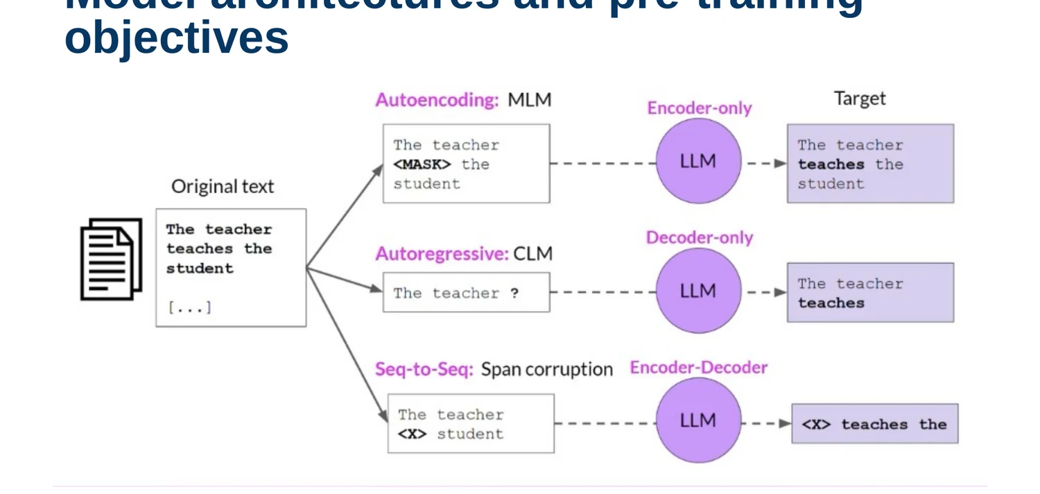
The architecture is not selected by a slogan such as “generative models are better.” Choose the information boundary and output interface the task needs. Code comments converted into executable code are naturally conditional generation; invoking a structured action from text is a separate application behavior. Translation is naturally sequence-to-sequence, although a sufficiently capable decoder-only model can also express it as prompted continuation. “Well suited” describes an inductive bias, not an absolute prohibition.

The Real Training Memory Budget

Parameters Are the Easy Part

For parameters stored with bytes each, weight memory is

One billion FP32 parameters therefore require approximately bytes, or about 4 GB in decimal units. A 175B model would require roughly 700 GB merely for FP32 weights. This estimate is useful for inference planning, but it badly underestimates training.

The word “approximately” matters. Framework metadata, tensor alignment, embeddings, buffers, temporary workspaces, and whether memory is reported in GB or GiB change the observed number. The formula is a first budget, not a promise that an allocator will fit the model into a device with exactly that capacity.

Adam Adds Persistent State

Training retains more than the current weights. A common FP32 accounting for Adam is:

Component	Approximate bytes per parameter
Model weights	4
Gradients	4
Adam first moment	4
Adam second moment	4
Activations and temporary buffers	variable

The two Adam moments already add 8 bytes per parameter. Some mixed-precision recipes also keep an FP32 master copy of weights while computing with FP16 or BF16, adding another 4 bytes. A useful high-end planning heuristic is roughly 24 bytes per parameter: 4 for weights, 8 for Adam states, 4 for gradients, and about 8 for activations and temporary memory. Under that heuristic, training 1B parameters can approach 24 GB rather than the 4 GB needed to store FP32 weights.

Do not treat 24 bytes as a universal constant. Optimizer choice, master weights, gradient precision, fused kernels, checkpointing, attention implementation, sequence length, microbatch size, and tensor parallelism all change it. The durable lesson is the ledger: name every resident tensor before claiming that a model fits.

Activations Depend on the Workload

Optimizer state scales mostly with parameter count. Activations scale with the computation being remembered for backpropagation. A rough Transformer activation budget grows with

where is microbatch size, sequence length, layer count, and hidden width. Ordinary attention can also create score tensors. Modern fused attention kernels may avoid materializing the full matrix, but longer context still increases computation and other stored states.

Activation checkpointing reduces memory by discarding selected intermediate values during the forward pass and recomputing them during backward. It trades extra FLOPs for a lower memory peak. Gradient accumulation reduces the microbatch that must fit at once while preserving a larger effective batch over several steps. These techniques solve different problems from parameter sharding.

A Budgeting Example

Suppose a 7B model uses BF16 weights for the forward and backward passes. The raw weight copy is roughly

That does not imply that a 16 GB GPU can train it. Gradients, optimizer states, possible master weights, activations, communication buffers, and allocator fragmentation remain. Conversely, inference may fit after quantizing weights to 8 or 4 bits because it does not retain backward activations or Adam states. This is why statements such as “the model is only 14 GB” are incomplete unless they name the operation: load, infer, fine-tune, or pretrain.

Precision, Mixed Precision, and Quantization

What a Floating-Point Format Stores

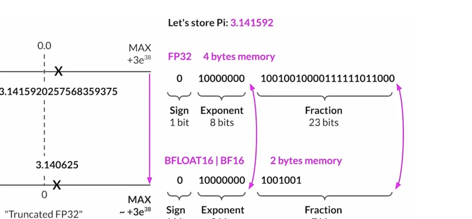
A floating-point number is represented by sign, exponent, and fraction fields. Ignoring special values, its magnitude behaves like

The exponent controls range; the fraction controls precision. This distinction explains why FP16 and BF16, although both occupy 16 bits, behave differently.

Format	Sign	Exponent	Fraction	Bytes	Practical meaning
FP32	1	8	23	4	wide range and good precision
FP16	1	5	10	2	more fraction precision than BF16, much narrower range
BF16	1	8	7	2	FP32-like range, coarser precision
INT8	signed integer	-	-	1	discrete levels with an external scale/zero point

The representation of makes the tradeoff visible. FP32 stores approximately , while a 16-bit format stores a coarser value. Fewer fraction bits mean larger gaps between adjacent representable numbers. Fewer exponent bits mean underflow or overflow happens sooner.

BF16 keeps FP32's 8-bit exponent but shortens the fraction, preserving range at the cost of precision. Course slide 38.

Why BF16 Is Popular for Training

Deep-network gradients can span a large dynamic range. FP16 has more fraction bits than BF16 but only a 5-bit exponent, so small gradients may underflow and large values may overflow unless loss scaling is handled carefully. BF16 retains the 8-bit exponent of FP32 and is therefore more forgiving, while cutting storage and memory bandwidth in half for tensors represented in BF16.

Mixed-precision training does not mean every operation blindly uses one low-precision format. A practical system may compute matrix multiplications in BF16, accumulate some reductions at higher precision, and keep optimizer updates or selected statistics in FP32. The goal is to place precision where it affects stability and use narrower formats where they improve throughput and capacity.

Quantization Is a Mapping, Not a File Conversion

For affine integer quantization, a real value can be mapped to an integer code

and approximately reconstructed as . The scale and zero point define which real interval the finite integer codes represent. Per-channel scales often preserve accuracy better than one scale for an entire tensor because different channels may have different ranges.

Lower precision reduces weight memory and memory traffic, but the gain depends on hardware and kernels. INT8 weights occupy one quarter of FP32 storage; 4-bit weights occupy one eighth. Yet dequantization metadata, unquantized layers, KV cache, activations, and temporary buffers remain. A file that is four times smaller does not guarantee a fourfold end-to-end speedup.

Post-Training Quantization and QAT

Post-training quantization chooses scales after training, usually with calibration data. It is inexpensive but can lose quality when distributions contain outliers or the target bit width is aggressive. Quantization-aware training (QAT) simulates quantization during training so the parameters adapt to its rounding and clipping error. QAT usually preserves more quality but requires additional training and engineering.

It is useful to keep three ideas separate:

• BF16 mixed-precision pretraining reduces memory and accelerates training while retaining floating-point behavior.
• Weight-only INT8 or 4-bit quantization often targets inference memory and bandwidth.
• QAT changes the training procedure so the final model tolerates a particular quantized representation.

The best format is therefore workload-specific. Ask which tensors are narrow, which operations have native hardware support, what accuracy loss is acceptable, and whether the bottleneck is memory capacity, bandwidth, arithmetic throughput, or communication.

From One GPU to Many

DDP Replicates the Model and Splits the Batch

Distributed Data Parallel (DDP) places a full model replica on each of workers. Each worker receives a different microbatch, computes a forward and backward pass, and produces a local gradient . A collective reduction forms the shared gradient,

after which each replica applies the same optimizer update. If every worker starts from the same parameters and receives the same reduced gradient, the replicas stay synchronized.

DDP is attractive because the expensive forward and backward computations happen in parallel. Gradient all-reduce can be bucketed and overlapped with backward computation. It also increases global batch size unless the per-worker batch is reduced:

where is the number of gradient-accumulation steps. Learning-rate schedules and optimization behavior may need adjustment when this value changes.

What DDP Does Not Solve

DDP requires every worker to hold a full copy of the weights, gradients, and optimizer state. It accelerates a model that already fits on one GPU; it does not make a too-large model fit merely by adding replicas. If one complete training state requires 120 GB, four 80 GB GPUs running ordinary DDP still each need roughly that state.

Communication also limits scaling. If one GPU finishes its computation early, it waits at synchronization points. Slow data loading, imbalanced batches, network topology, small per-GPU work, and collective latency can leave expensive accelerators idle. More GPUs reduce wall-clock time only while useful compute outweighs added communication and coordination.

ZeRO Removes Replicated State

The Zero Redundancy Optimizer asks why every data-parallel rank must store identical training state. With workers, sharding ideally reduces a sharded component’s per-worker footprint by roughly :

• ZeRO Stage 1: shard optimizer states.
• ZeRO Stage 2: shard optimizer states and gradients.
• ZeRO Stage 3: also shard model parameters.

ZeRO progressively removes redundant copies: optimizer states first, then gradients, then parameters. Course slide 57, based on Rajbhandari et al.

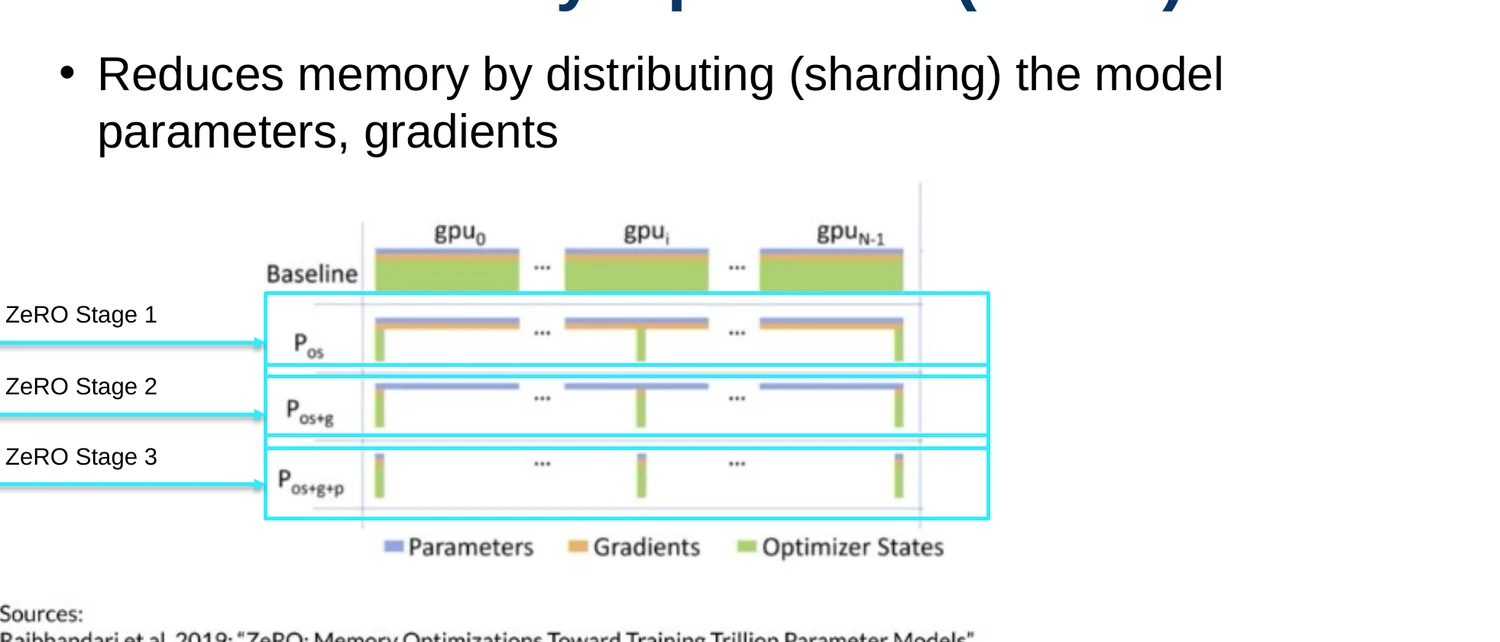
The gain is not free. A rank that owns only a shard must communicate when computation needs the full logical tensor. Sharding changes a capacity problem into a communication-and-scheduling problem. The network, tensor grouping, prefetch schedule, and overlap with computation determine whether the trade is worthwhile.

FSDP Reconstructs One Block at a Time

Fully Sharded Data Parallel (FSDP) implements the full-sharding idea around modules or parameter groups. Conceptually, for each wrapped block:

1. parameters are stored as shards while idle;
2. an all-gather reconstructs the block’s parameters before its forward computation;
3. full parameters can be discarded or reshared after use;
4. they are gathered again when backward needs them;
5. gradients are reduce-scattered, so each rank retains only its shard;
6. the optimizer updates the local parameter and optimizer-state shards.

Fine-grained groups lower peak memory and allow communication for the next block to overlap with computation on the current block. Groups that are too small create many inefficient collectives; one giant group creates a large blocking all-gather and high memory peak. Wrapping policy is therefore a performance decision, not only an API detail.

CPU offload can move parameters or optimizer state out of GPU memory, making otherwise impossible runs fit. It also adds transfers over a much slower link. Offload is a capacity escape hatch, not guaranteed acceleration.

Capacity and Throughput Must Be Measured Together

FSDP can enable much larger models, but weak scaling is not automatically linear. PyTorch FSDP results comparing full sharding, hybrid sharding, full replication, and DDP show per-GPU throughput declining as the number of 80 GB A100s grows for a fixed large model. That decline is the cost of coordination and reduced compute per participant.

Sharding expands feasible model size, but communication and parallel efficiency still determine useful throughput. Course slide 65, after Zhao et al.

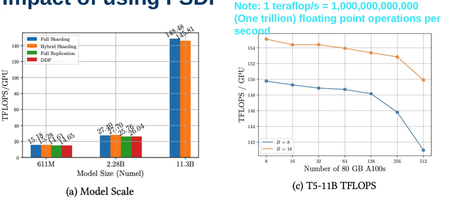
Always record at least peak memory, samples or tokens per second, model FLOP utilization, communication time, and convergence quality. A configuration that fits but spends most of its time in collectives is not an efficient training system.

Compute Budgets and Scaling Laws

Turn Hardware Time into Compute

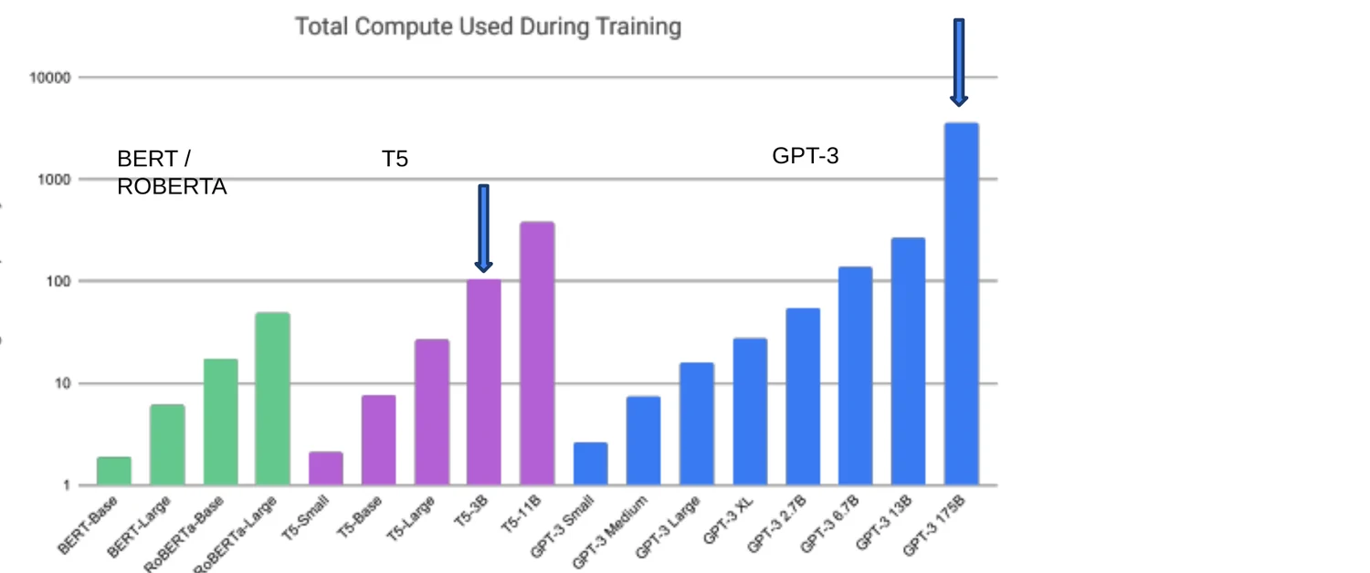
A petaflop/s-day is the work performed by one sustained petaflop per second for one day:

This is a unit of work, not a promise about elapsed time. If eight accelerators each advertise a peak rate, the achieved rate is lower unless kernels, memory, communication, and scheduling keep them fully utilized. Training cost can be approximated as achieved compute multiplied by wall-clock time, or estimated from model and token counts.

For a dense decoder Transformer, a frequently used first-order estimate is

where is the number of non-embedding parameters and is the number of training tokens. The factor accounts roughly for forward and backward matrix operations. Attention, embeddings, sparsity, sequence length, recomputation, and implementation details make it an approximation.

Historical pretraining runs differ by orders of magnitude in total compute; parameter count alone does not reveal the training bill. Course slide 69.

Scaling Laws Are Empirical Forecasts

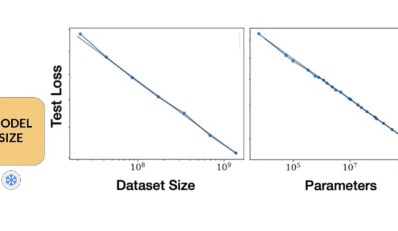
Scaling studies fit relationships among loss , model size , data size , and compute . A simplified form is

with fitted constants that depend on architecture, data, tokenizer, and training setup. The curve says that more parameters or data usually reduce loss with diminishing returns. It does not say that every dataset is equally valuable or that benchmark quality is completely determined by token count.

The practical use is planning. Train smaller models across multiple sizes and token budgets, fit an empirical frontier, and forecast which larger configuration is worth attempting. Extrapolation is uncertain; it should be accompanied by confidence ranges and checkpoints that can stop a bad run early.

Loss often follows a near-linear trend on log-log plots over a measured regime, which motivates empirical scaling forecasts. Course slide 72.

Fixed Compute Creates an Allocation Problem

Under a budget, a larger model processes fewer tokens; a smaller model can train longer. Using , holding fixed means is approximately fixed. Neither extreme is optimal:

• too small a model may lack capacity even after many tokens;
• too large a model may be undertrained, seeing too little data to learn its parameters well.

For each compute level, an IsoFLOP experiment trains several model sizes with token counts chosen to keep total compute similar. Final loss typically forms a valley. The bottom of that valley estimates the compute-optimal allocation. This is a stronger method than plotting one training run per model size and assuming the largest parameter count caused the best result.

Kaplan and Chinchilla Changed the Allocation

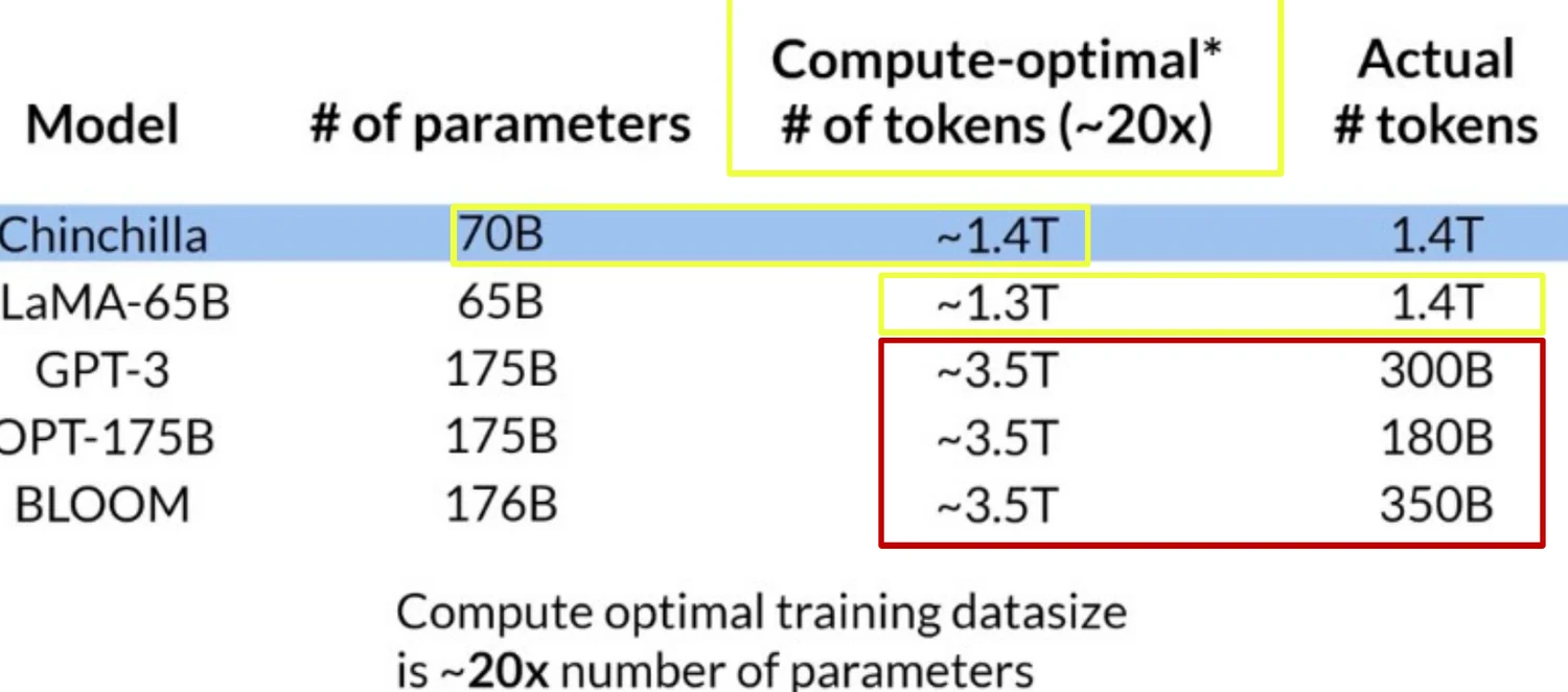
Earlier scaling guidance emphasized growing parameter count faster than dataset size. The Chinchilla study trained more than 400 models and found a substantially different compute-optimal frontier: model size and token count should grow in approximately equal proportions with compute,

Its central demonstration compared Gopher, 280B parameters, with Chinchilla, 70B parameters trained on 1.4T tokens at the same compute budget. The smaller, more thoroughly trained model performed better across many evaluations and was cheaper to serve. The lesson is not “70B is always ideal”; it is that a huge model can be over-parameterized for its training budget.

The often quoted “about 20 tokens per parameter” is a rule derived from a particular compute-optimal analysis, not a timeless constant. Course slide 77.

Batch Size Is Related but Not Interchangeable

A complete scaling checklist includes batch size, model size, dataset size, and compute budget. They affect different layers. and allocate total learning capacity and exposure. Batch size controls how many tokens contribute to one optimizer step, affects gradient noise and hardware utilization, and determines the number of updates for a fixed token budget.

Doubling the batch does not double the information in a fixed dataset, and a batch can become so large that optimization quality stops improving. Separate microbatch size (what fits on a worker), global batch size (all workers and accumulation), and training tokens (all examples consumed across the run). Tuning one does not erase constraints on the others.

Domain Pretraining

Specialized Language Changes the Distribution

Medical, legal, and financial text contains ordinary words used in specialized ways, rare terminology, compact notation, and domain-specific relationships. “Consideration” in contract law, qid pc & hs in a prescription, and a ticker symbol in a market report carry meanings that general conversational data may underrepresent.

A domain model must therefore answer two questions:

1. Does the tokenizer represent the domain efficiently?
2. Does the training distribution expose the model to enough examples of the domain’s concepts, tasks, and writing styles?

Retrieval can supply a missing current fact, but it does not completely replace domain representations. Conversely, domain pretraining does not replace retrieval for rapidly changing prices, filings, or regulations. One changes the model’s parameters; the other changes the evidence available for the current answer.

Choose a Data Strategy

There are three common strategies.

General pretraining followed by domain-adaptive pretraining is economical because it reuses broad language ability. It risks forgetting or shifting general capabilities if the domain stage is too narrow or aggressive.

Joint pretraining on a mixed corpus learns domain and general language together. Mixture weights become critical: dataset size is not the same as sampling probability, and repeated small sources may influence the model more than raw token counts suggest.

Domain-only training from scratch offers maximum control but may produce a model that is excellent inside the domain and unnecessarily weak elsewhere. Most real financial workflows still contain ordinary instructions, news, dates, code, and conversational requests, so general competence remains useful.

Data Quality Is Part of the Objective

Before training, documents must be licensed, normalized, deduplicated, filtered, and split so evaluation data does not leak into pretraining. Personally identifiable or confidential material needs explicit governance. Temporal splits matter in finance: a model evaluated on information that already appeared in its corpus is not demonstrating forecasting or future generalization.

Mixture design should be recorded as both prepared tokens and expected consumed tokens. A 100B-token source sampled at 20% during a 500B-token run contributes roughly 100B draws, or about one epoch, before accounting for filtering and packing. Without sampling weights and epochs, a corpus table does not fully describe what the model learned from.

BloombergGPT: Design and Training

Two Requirements, One Model

BloombergGPT is a 50B-parameter causal language model designed to be strong on financial tasks without giving up general-language performance. Those requirements pull in different directions. A purely general model may not represent filings, market shorthand, ticker links, or Bloomberg Query Language well. A purely financial model may lose broad reading comprehension and instruction vocabulary.

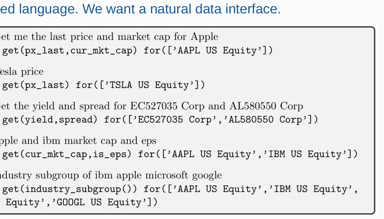
The paper’s BQL example makes the product motivation tangible: a user writes a natural request about prices, market capitalization, or industry groups, and the model generates an executable-looking query. The figure demonstrates three-shot query generation, not verified query execution. A production system would still parse, authorize, and test the generated query.

A financial language interface changes specialized requests into BQL-like output; generation and safe execution remain separate stages. Course slide 87, adapted from BloombergGPT Figure 4.

Prepared Corpus Versus Consumed Tokens

The prepared corpus contains about 708.9B tokens: approximately 363B financial tokens and 345B general-purpose tokens. FinPile accounts for 51.27% and public general data for 48.73%. FinPile includes web material, financial news, filings, press releases, and Bloomberg material; it should not be described as entirely private. General sources include The Pile, C4, and English Wikipedia.

The selected checkpoint did not consume all 708.9B prepared tokens. It was chosen at step 139,200 after about 569B consumed tokens. Prepared capacity and actual training exposure are different quantities. This distinction prevents a common error: reading a corpus total as if every token were necessarily used exactly once.

The mixed corpus is also evidence about the design goal. Roughly half financial and half general text is an attempt to balance specialization with broad competence. It does not, by itself, prove that this particular ratio caused the final scores; a causal claim would require controlled mixture ablations.

Tokenizer and Causal Objective

BloombergGPT uses a Unigram tokenizer trained on a broad corpus. The design permits multi-word tokens and retains token probabilities during tokenizer construction; spaces can remain inside pieces. Numbers are split into chunks, motivated by the hope that structured numeric fragments are easier to represent than arbitrary long strings.

Tokenizer efficiency is a systems concern as well as a linguistic one. If a domain expression takes fewer tokens, more information fits into a 2,048-token context and training spends fewer token positions on the same document. A larger vocabulary, however, enlarges the input embedding and output projection and can leave rare vocabulary items poorly trained. “Denser tokenization” therefore has a model-memory and data-frequency cost.

Documents are tokenized, concatenated with separators, packed into 2,048-token chunks, and trained with causal next-token prediction. At position , only tokens through can predict token . BloombergGPT is therefore not trained with BERT-style masking or T5-style span corruption, even though all three are self-supervised objectives.

Model Size Under a Real Budget

The team did not simply choose the largest parameter count that could be named. Available financial data and compute constrained the allocation. The BloombergGPT analysis compares earlier Kaplan guidance with Chinchilla-style estimates: near the available compute budget, Chinchilla suggests fewer parameters and more tokens than the earlier frontier.

BloombergGPT lies near a budget where competing scaling-law fits recommend materially different parameter/token allocations. Course slide 94, adapted from BloombergGPT Figure 1.

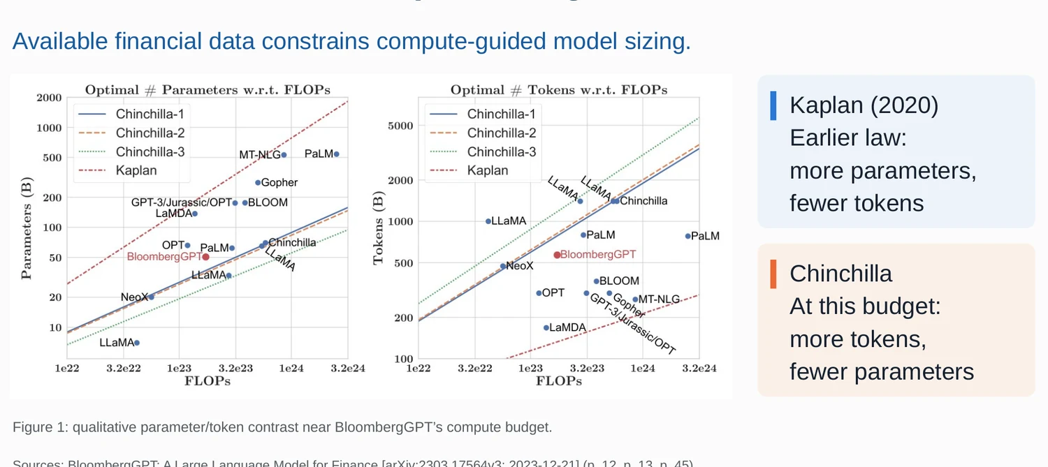
This choice illustrates why scaling laws are planning tools rather than commands. The corpus has domain constraints, the fitted laws come from other model families and data, and operational goals include inference cost as well as training loss. A 50B model trained on hundreds of billions of tokens represents a compromise among empirical scaling forecasts, available financial data, and the system the team could train.

ZeRO, MiCS, Mixed Precision, and the Checkpoint

Three implementation choices solve different costs:

• ZeRO Stage 3 shards parameters, gradients, and optimizer state.
• MiCS organizes sharding and communication for cloud-scale clusters, reducing expensive cross-node traffic.
• Mixed precision uses BF16 for memory-efficient computation while retaining FP32 where stable updates require it.

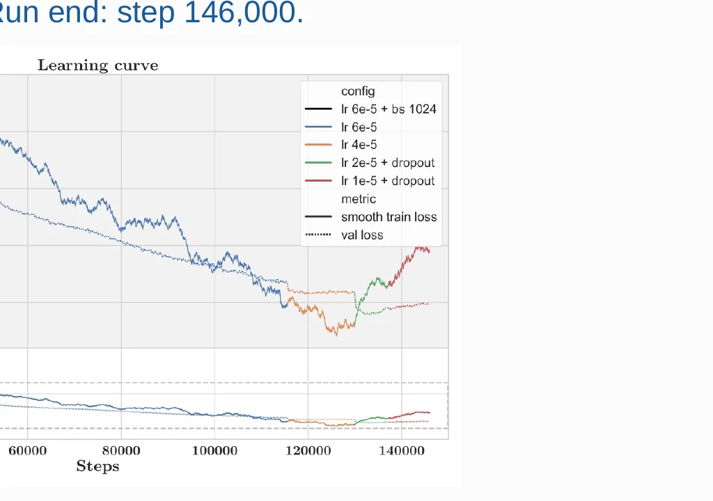
The successful training path improved for most of the run and then plateaued. The selected checkpoint is step 139,200 with 569B consumed tokens; the run ended at step 146,000. The curve is valuable because it makes checkpoint selection an evidence problem. The last written checkpoint is not automatically the best one, especially when validation loss or stability deteriorates.

The retained checkpoint precedes the end of the run; “latest” and “best validated” are different policies. Course slide 96, adapted from BloombergGPT Figure 2.

BloombergGPT: Evaluation and Evidence

Compare Tasks Before Comparing Models

The evaluation suite contains three families:

• public finance: sentiment, headline classification, ConvFinQA, and named-entity recognition;
• internal finance: sentiment, entity spans, and company-ticker prediction;
• general language: MMLU, BIG-bench Hard, reading comprehension, and linguistic tasks.

Shared evaluation inputs do not mean shared pretraining histories. GPT-NeoX, OPT-66B, BLOOM-176B, and BloombergGPT differ in architecture, data, token budgets, and training procedures. A table establishes performance under the reported protocol; it does not isolate which one design choice caused the difference.

Candidate Scoring Changes Multiple-Choice Results

For candidate answer and context , the paper considers several ranking rules. Regular scoring uses . Calibration divides by a baseline probability such as , reducing a candidate’s context-independent preference. Length normalization compensates for the fact that multiplying token probabilities tends to penalize longer candidates:

These rules can rank the same candidates differently. Reporting the best rule for each model/task improves a model’s displayed result relative to committing to one universal scoring rule, so the protocol must be read alongside the number.

Financial Results Are Strong but Not Uniform

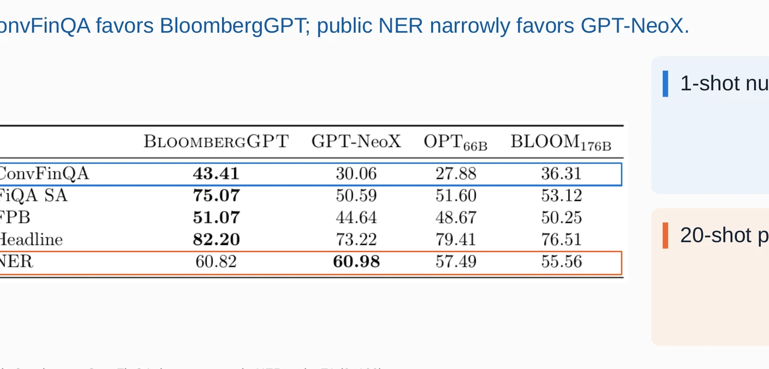
On the highlighted public financial rows, BloombergGPT leads FiQA sentiment, Financial PhraseBank sentiment, and headline tasks. The metrics are F1-based, not ordinary accuracy. For binary or multiclass predictions, F1 balances precision and recall; in its binary form,

BloombergGPT leads several finance rows, but every row must be read with its own metric and prompting setup. Course slide 99, adapted from BloombergGPT Table 8.

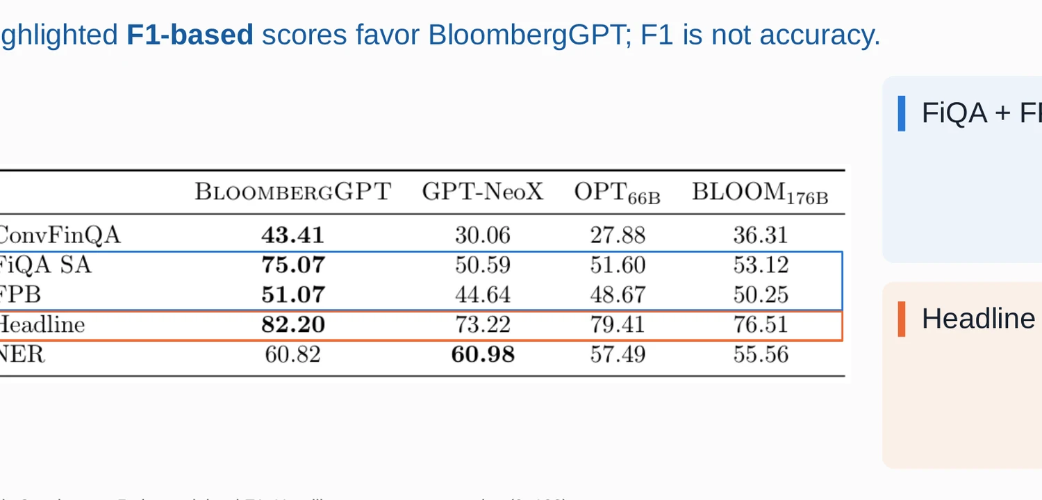
There are explicit exceptions. BloombergGPT performs strongly on one-shot ConvFinQA numerical question answering, while GPT-NeoX narrowly leads the reported public NER row. Internal sentiment gains also vary: the lead is large for some news datasets and much closer for equity social media. A credible conclusion preserves these exceptions instead of replacing the whole table with “the domain model wins.”

Domain specialization improves many tasks, not every task. ConvFinQA and public NER point in different directions. Course slide 100.

NER and Ticker Prediction Are Different Targets

Named-entity recognition extracts typed spans. From “Steve Jobs is the CEO of Apple,” a strict NER system may return Steve Jobs as a person and Apple as an organization. Exact-match evaluation can count a boundary error as wrong even when the phrase is almost correct.

Ticker prediction adds entity disambiguation. Given “AAPL announced it would stop using Intel chips,” an NER output may identify AAPL and Intel; an NER-plus-NED system maps them to AAPL and INTC. The target has changed from locating mentions to resolving mentions against a financial identifier space. Strong performance on one should not be silently reported as performance on the other.

This is a broader evaluation lesson: write down the unit of prediction, allowed output, matching rule, and averaging method before interpreting a score. “Entity F1” without those details is incomplete.

General Capability Has Boundaries Too

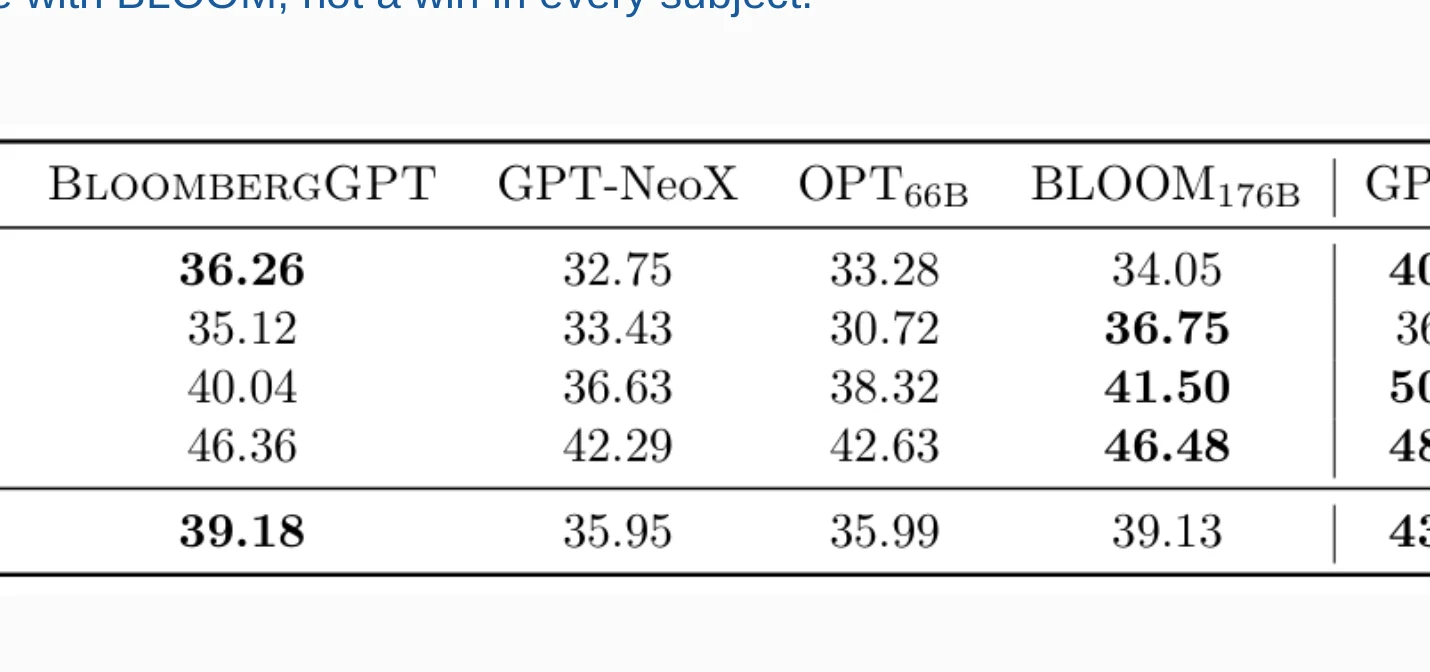
BloombergGPT’s reported five-shot MMLU average, 39.18, is very close to BLOOM-176B’s 39.13, but the subject rows vary. A near tie in the mean does not mean the models behave identically in humanities, STEM, social science, and other subjects. GPT-3’s displayed numbers come from an external result rather than the same author-run pipeline, which further limits direct comparison.

Broad competence is not one number: BloombergGPT is near BLOOM on the reported MMLU mean while individual subject groups differ. Course slide 104, adapted from BloombergGPT Table 15.

On BIG-bench Hard, the reported average is 41.97 for BloombergGPT and 44.91 for BLOOM-176B; BloombergGPT still exceeds the displayed NeoX and OPT averages. This is evidence for a balance—strong financial performance with competitive general ability—not proof that specialization is free or that the model is best on every general task.

What Pretraining Does Not Finish

Findings Versus Causal Claims

The results support a careful statement: the trained 50B model performs strongly on the tested financial suite while remaining competitive on the reported general benchmarks. They do not establish that the 51/49 mixture is uniquely optimal, that the tokenizer caused the gains, or that the model is safe for autonomous financial decisions. Those questions need ablations, calibration, robustness tests, and deployment-specific evaluation.

Benchmark scores also do not reveal data freshness, memorization, fairness across users, resistance to adversarial instructions, or the cost of a wrong action. Financial applications need access controls, current data, audit logs, numerical verification, and often human approval in addition to a capable pretrained model.

Open Technical Questions

Several directions remain investigations rather than completed improvements:

• test financial instruction alignment and task fine-tuning;
• measure toxicity and bias at the model level, not only the dataset level;
• isolate how the tokenizer affects the resulting model;
• explore a longer stable run and alternatives such as SwiGLU, RoPE, and query/key normalization;
• compare joint pretraining with general pretraining followed by domain adaptation;
• improve sample efficiency and study post-training conditioning.

Each item belongs to a different experiment. For example, changing the tokenizer alters sequence lengths, vocabulary parameters, and data packing simultaneously. A fair comparison must hold the relevant compute or token budget constant and record the new denominator.

A Pretraining Decision Checklist

Before approving a large run, be able to answer these questions:

1. Objective: What is predicted, and what context is visible?
2. Data: What sources are allowed, how are they filtered and deduplicated, and what mixture will actually be sampled?
3. Tokenizer: How efficiently does it represent the important languages, numbers, code, and domain terms?
4. Budget: What are , , sequence length, global batch, expected FLOPs, wall-clock time, and cost?
5. Memory: Which tensors are replicated, sharded, recomputed, quantized, or offloaded?
6. Parallelism: Why DDP, ZeRO/FSDP, tensor parallelism, pipeline parallelism, or a hybrid?
7. Precision: Which tensors use FP32, BF16, FP16, INT8, or lower precision, and how will numerical stability be monitored?
8. Checkpoints: Which validation signal selects the checkpoint, and how will the run recover from failure?
9. Evaluation: Which domain, general, safety, and operational tests define success, and what are their exact metrics?
10. Deployment: Can the selected model meet inference memory, latency, throughput, privacy, and governance constraints?

If one of these answers is “we will decide after training,” it may be the most expensive unresolved requirement in the project.

The main idea of this blog is not that every useful LLM must become larger. It is that pretraining is an allocation problem under evidence and constraints. The objective determines what signal the model receives. Precision and sharding determine whether the state fits and moves efficiently. Scaling laws help divide compute between parameters and tokens. Data mixture determines which distributions the model repeatedly sees. Evaluation then tells us what the resulting system can support—and, just as importantly, what it has not established.

References

• BloombergGPT: A Large Language Model for Finance
• Training Compute-Optimal Large Language Models
• ZeRO: Memory Optimizations Toward Training Trillion Parameter Models
• PyTorch Fully Sharded Data Parallel documentation

References

- Title: LLM 5 - Pretraining, Scaling, and Domain Models
- Author: Gavin0576
- Created at : 2026-10-09 18:00:00
- Updated at : 2026-10-09 20:42:45
- Link: https://jiangpf2022.github.io/blog/2026/10/09/LLM-5-Pretraining-Scaling-and-Domain-Models/
- License: This work is licensed under CC BY-NC-SA 4.0.