LLM 2 - Attention and Transformers

Welcome back. In LLM 1 we asked what makes deep learning possible as a statistical and computing system. Today we open the model itself. How does a token acquire meaning from its neighbors? How can a network decide which earlier words matter? Why did the Transformer replace recurrence for so many language tasks? And what actually separates BERT, GPT, and a mixture-of-experts model?

The lecture slides revisit the same mechanism through several diagrams. Here I have merged the repeated views into one line of reasoning. We will start with a deliberately simple representation, discover what it cannot express, build attention one operation at a time, and then assemble the complete architecture. Historical model tables appear near the end, where their dimensions and data mixtures have a reason to matter. The diagrams are cropped from the course slides and placed beside the concepts they illustrate; the equations and examples below are written out so that you can work through them yourself.

Word Representations

From IDs to Vectors

A language model cannot directly multiply the English word “cat” by a weight matrix. It first turns text into tokens, gives each token an integer ID, and looks up a numeric vector. The most literal vector representation is one-hot: if the vocabulary contains tokens, token becomes a vector in with a at position and everywhere else. One-hot vectors identify tokens perfectly but say nothing about similarity. Distinct tokens have dot product zero whether they mean “kitten” and “cat” or “kitten” and “thermostat.” They are also wasteful when is large.

Instead, learn a matrix , with . The vector for token is row . This embedding can reflect regularities found in the training data. Nearby vectors may represent words used in similar contexts; the network is free to change the coordinates as training proceeds. An embedding is therefore a learned representation, not a dictionary definition.

A one-hot basis separates IDs; a learned embedding space can express similarity. Course slide 3.

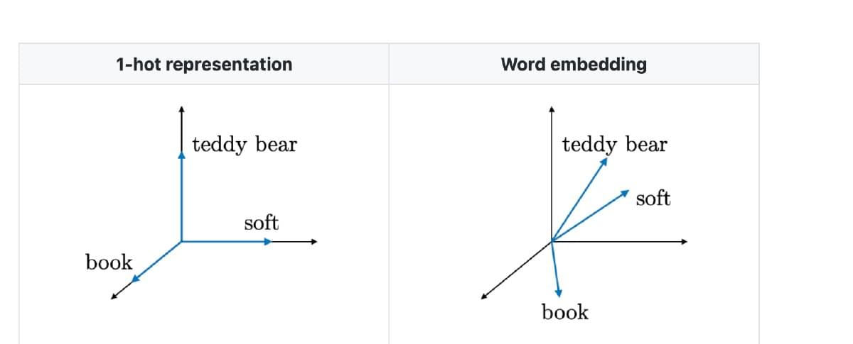
The Word2Vec heatmap in the slides is one visualization of learned dimensions. Its colors are coordinates of different word vectors, not hand-labeled semantic traits. We can compare vectors with cosine similarity,

but high similarity means “close under this model and training corpus,” not “interchangeable in every sentence.” Context, frequency, domain, and tokenization all influence the geometry.

Word2Vec and Analogies

Word2Vec learns vectors from a prediction problem built out of nearby text: depending on the variant, predict a context from a center word or predict a center word from its context. The surrounding words supply the supervision, so no human has to attach a separate semantic label to each example. The lecture’s famous arithmetic is

Read this as an observed geometric pattern: the displacement from man to king can resemble the displacement from woman to queen. We would compute the left side and find its nearest vocabulary vector. It is not an algebraic law of language; analogies depend on the corpus, model, and relation. They are useful precisely because they show that training can organize semantic and syntactic patterns without explicitly coding them.

The larger lesson is that representation learning changes the problem the next layer sees. A classifier given one-hot IDs must discover every useful relationship from scratch. A classifier given informative embeddings can exploit relationships already present in the vectors. This is why pretrained representations became central to transfer learning.

Why Static Vectors Fail

Word2Vec gives one stored vector to each vocabulary item. That vector cannot fully express a word whose role changes with the sentence. The slides use two versions of a sentence: “The chicken didn’t cross the road because it was too tired” and “… because it was too wide.” In the first, it plausibly refers to the chicken; in the second, to the road. A fixed vector for it is identical in both cases. It may encode general properties of pronouns, but it cannot itself encode which antecedent is intended here.

There are other kinds of ambiguity: bank can be a financial institution or a river edge; cold can describe temperature or an illness. A contextual representation should be a function of both the token and its sentence,

so two appearances of the same token can produce different . Do not confuse the input lookup vector with the final contextual hidden state . The former is fixed for that ID within a given model checkpoint; the latter changes when its neighbors change.

ELMo: Context Before Transformers

ELMo, Embeddings from Language Models, is an important bridge from static word vectors to contextual representations. It uses recurrent networks—specifically forward and backward LSTMs—to process the sentence in both directions. At position , a forward state has seen tokens ; a backward state has seen . Together they provide left and right context. The course diagram shows two directions and the layers between token embeddings and word-prediction outputs.

Forward and backward language-model states supply context from both sides of each word. Course slide 9.

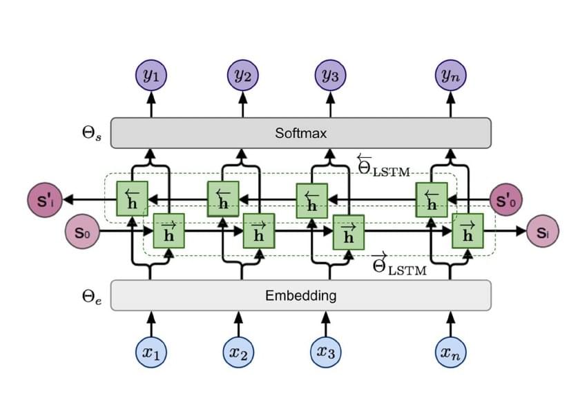
Why can this be trained without labeled sentiment or entity data? A sentence is its own source of targets. The forward language model predicts the next token from its prefix; the backward model predicts a token from its suffix. A simplified training objective is

The forward and backward models are trained with their own directional objectives; their internal states are then combined into a representation for a downstream task. ELMo does not have to use only its top layer. If is an initial token representation and are bidirectional layer states, a task can learn weights and a scale :

Different layers can contribute different information. A named-entity recognizer may value different features than a sentiment classifier. ELMo therefore makes two ideas concrete: pretrain on unlabeled text, then reuse context-sensitive states for a separate task. Its limitation for our next step is that recurrent processing still passes information through sequential state updates. Attention offers a more direct route between distant positions.

Attention

Why Selective Context Matters

Consider the slide pair “The cat drank the milk because it was hungry” and “The cat drank the milk because it was sweet.” The token it is the same. The useful evidence changes: hungry points toward the cat, while sweet points toward the milk. A good contextual representation should select relevant earlier words rather than treating every word as equally important.

The salient earlier word changes with the sentence continuation. Course slide 13.

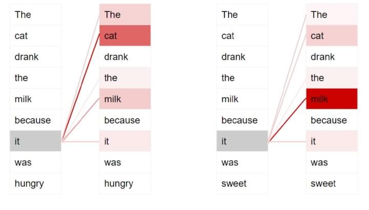
Attention implements this idea as a weighted sum. For a current position , assign scores to candidate context positions , turn scores into nonnegative weights that sum to one, and average their information vectors. In the simplest pedagogical version, the score could be and the value could be the original vector . This is helpful intuition but too restrictive: the features useful for finding information need not be the same as the information we want to retrieve.

Queries, Keys, and Values

That distinction produces the three roles in an attention head. A query states what the current position is looking for. A key advertises what a candidate position might provide. A value is the content transferred if the candidate receives weight. They are learned projections of the input vectors:

If , then and . Thus and . The score is a compatibility measure,

is the set of positions allowed for query . In a bidirectional encoder it may include the whole sentence; in a causal decoder it includes only positions up to . The denominator keeps dot-product magnitudes from growing with key dimension. Without scaling, large scores can drive the softmax toward a near-one-hot distribution too early, leaving weak gradients for most alternatives.

The numbers are attention weights, not probabilities that a pronoun “truly means” a particular noun. They tell us how this head combines value vectors at this layer. Different heads and later layers may behave differently; a vivid heatmap should not be mistaken for a complete causal explanation of the model.

One Head, Step by Step

Let us calculate a tiny causal head. Suppose the query at position has legal keys , and its scaled scores are . Exponentiating yields , so softmax gives weights . If the corresponding scalar values are , the attention output is

We did not choose the third value simply because its score was highest. The output is a weighted combination; the largest weight happens to multiply zero. With vector values, exactly the same arithmetic applies coordinate by coordinate. This distinction—scores choose weights; values supply content—prevents many errors when reading attention diagrams.

At position 3: project Q/K/V, compare the query with legal keys, scale, softmax, weight values, and sum. Course slide 24.

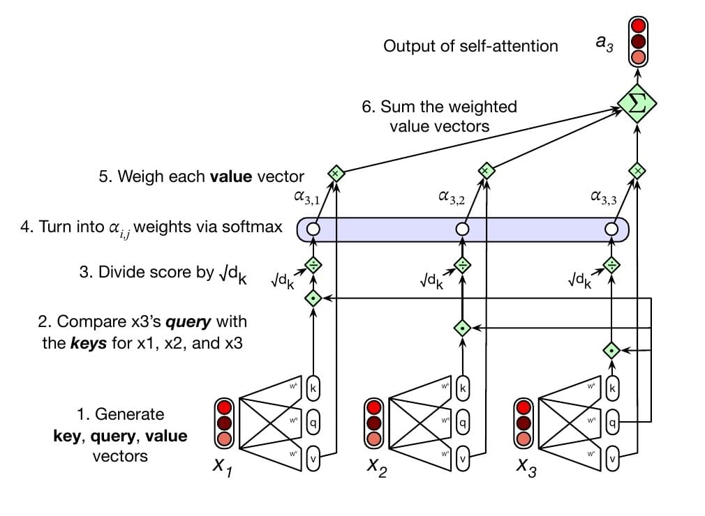
In a left-to-right language model, the legal set excludes positions onward. If we let training look at a future token while predicting it, the task would leak its own answer. The causal mask is therefore a condition of the prediction problem, not a cosmetic choice. An encoder intended to understand an already available sentence usually does not need this future mask.

Multi-Head Attention

One head learns one set of projections and produces one weighted summary. With heads, we repeat the calculation using different learned matrices, concatenate the outputs, and project back to model width:

If each head has value width , concatenation has width , so returns to the -dimensional residual stream. The slides draw eight heads as an example, not as a universal requirement. Different heads can learn different comparisons or positions, although they are not guaranteed to correspond neatly to human concepts such as “syntax head” and “pronoun head.”

Each head has its own projections; concatenation and recombine their outputs. Course slide 26.

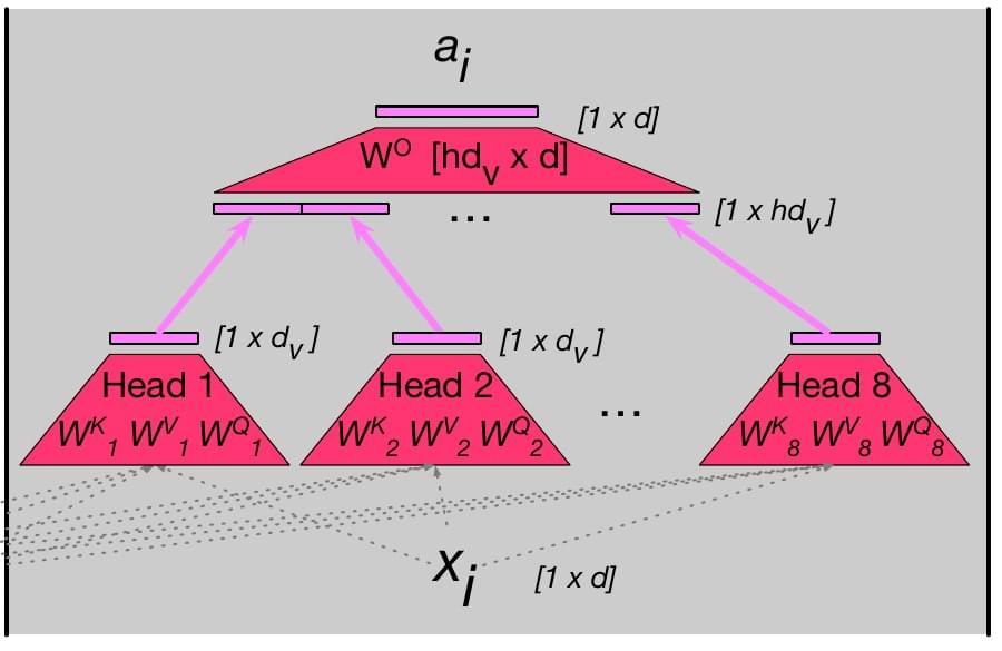
The important achievement is not that the model has many “opinions.” It is that each token can request information directly from other tokens, and the weighted information can enter its representation in one layer. That idea arose before the Transformer, in sequence-to-sequence translation.

From Seq2Seq to Transformers

The Recurrent Bottleneck

A classic sequence-to-sequence model encodes an input sentence with an RNN, LSTM, or GRU, then uses a decoder to produce an output sentence one token at a time. In its simplest form, the decoder receives only the encoder’s final hidden state as its source summary. The encoder has to compress a variable-length sentence into one fixed-width vector. The decoder then has to recover the right details from that compressed vector at every output step.

Think about translating a long sentence whose first and last clauses both contain important names. A single final state must preserve word identities, order, and grammatical relationships while also supporting the next output decision. It can work, but the information bottleneck becomes increasingly uncomfortable as input length grows. The decoder’s own recurrent hidden state carries past output information; that does not by itself restore details lost from the source summary.

Attending to Encoder States

Attention-based seq2seq relaxes the bottleneck by retaining all encoder states . At decoder step , the decoder state supplies a query and scores those source states. It constructs a step-specific context vector,

then uses to help predict the next output token. Early attention mechanisms by Bahdanau, Cho, and Bengio and later Luong, Pham, and Manning developed useful versions of this idea. Bahdanau-style additive scoring and Luong-style multiplicative/global-or-local scoring differ in implementation, but both let the decoder consult a changing part of the source rather than one unchanging summary.

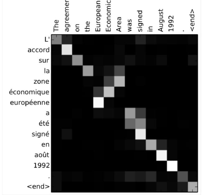
The slide’s alignment matrix illustrates this change. Bright cells indicate source positions receiving more weight at a particular output step. When English and French reorder a phrase, a decoder can shift its attention accordingly. The matrix is a soft alignment, not a hand-authored word-by-word dictionary.

A translation decoder can attend to different source positions at different output steps. Course slide 32.

Three Kinds of Transformer Attention

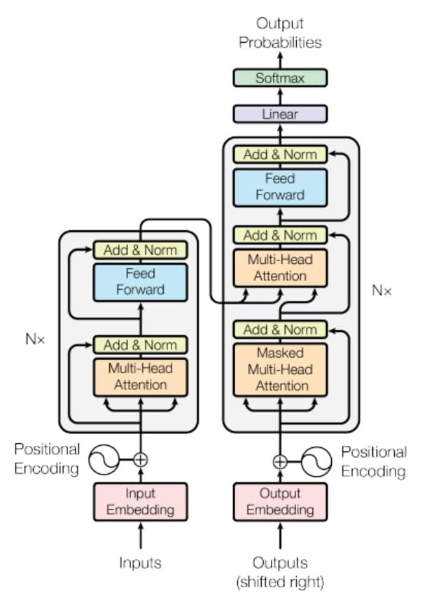
The 2017 Transformer kept the useful attention idea but removed the recurrent state update from the core encoder–decoder architecture. It uses three attention patterns that are easy to mix up:

Location	Queries come from	Keys and values come from	Visibility
Encoder self-attention	Encoder states	Encoder states	All unmasked source positions
Decoder self-attention	Decoder states	Decoder states	Current and earlier target positions only
Encoder–decoder cross-attention	Decoder states	Encoder outputs	Available source positions

The word self means the query, key, and value sequences originate from the same side. It does not mean a token attends only to itself. Cross-attention means the target-side query reads source-side representations. The original Transformer stacks attention, a position-wise feed-forward network, residual connections, and normalization. The decoder receives output tokens shifted right during training, so at position it is asked to predict the following token using only the preceding target prefix.

The original encoder–decoder Transformer has self-attention on both sides and cross-attention only in the decoder. Course slide 33.

What Parallelism Really Means

Without recurrence, the encoder can compute representations for all input positions in parallel within a layer. With shifted targets and a causal mask, decoder training can likewise score many target positions simultaneously: the correct previous tokens are already known. At generation time, however, the next token is not known until the current one has been produced. Autoregressive decoding remains sequential across output positions, even though operations within each step can be parallelized and previously computed keys and values can be cached.

This distinction explains both the Transformer’s training advantage and a persistent inference constraint. Attention makes distant positions directly reachable and maps well to matrix hardware, but its all-pairs interaction has a cost we can see once we write the operation in matrix form.

Attention as Matrix Computation

Shapes Before Arithmetic

Put token representations into a matrix , one token per row. Instead of invoking the same learned projections separately for every position, multiply whole matrices:

Then . Entry is exactly the query–key dot product from the previous section. Apply softmax across each row, because row represents the alternatives available to query . The result is an weight matrix ; multiplying produces outputs. This is the same weighted-sum operation as before, now expressed in matrix operations that accelerators handle efficiently.

Reading the dimensions from left to right prevents accidental transposes. Course slide 40; the equation is written explicitly in the text.

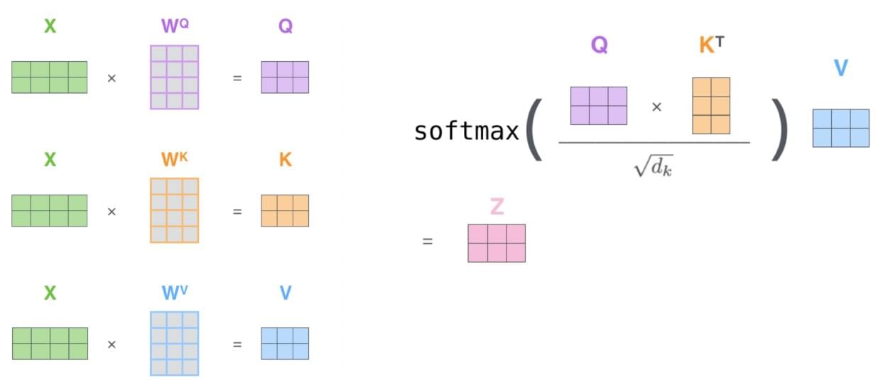
For cross-attention, do not force the source and target lengths to be equal. If decoder queries have length and encoder outputs length , then , have rows, the score matrix is , and the output has rows. That is why a translation decoder can make a different source summary for each target position.

Masking the Future

For causal self-attention, add a matrix before softmax:

where if and if . Since , every future position gets weight zero. In actual floating-point code a very negative finite value or a masked-softmax kernel may be used instead. The semantic requirement is the same: a query at time cannot read keys from onward.

The upper triangle is inaccessible to a left-to-right decoder. Course slide 48.

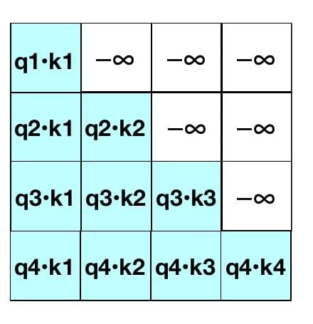
There may also be a padding mask. If a batch contains shorter sentences padded to a common length, the model should not attend to artificial pad tokens. Padding and causality solve different problems: the first excludes non-data positions; the second excludes future data positions. A bidirectional encoder typically uses padding but not a causal mask.

Why Sequence Length Is Expensive

compares every one of queries with every one of keys, so one ordinary self-attention head needs score arithmetic and an score or weight structure. Doubling sequence length roughly quadruples the number of query–key pairs. This is the quadratic-in-length point made in the lecture. Matrix kernels can be very fast, and implementations may avoid storing the full weight matrix, but the all-pairs interaction still places pressure on computation and memory. Other parts of the model, including the position-wise feed-forward network, have different scaling.

Do not turn this into the false claim that “Transformers are always slow for long text.” The comparison depends on sequence length, model width, hardware, kernels, batching, and whether we are training or generating. Recurrent models have a smaller interaction footprint per step but a sequential dependency across steps. Attention trades that recurrence for wider parallel work and direct access to distant tokens.

All Heads at Once

The slide first describes one triple and then several heads. In an implementation, the head projections are usually computed in large fused or batched operations. Conceptually, head has and computes

The head outputs concatenate along the feature dimension, then maps back to width . If , , and all heads share a -dimensional value width, concatenation has features before . The specific split is an architecture choice. The mask applies separately to every causal head; having more heads never grants access to forbidden future positions.

Inputs and Outputs

Tokenization and Lookup

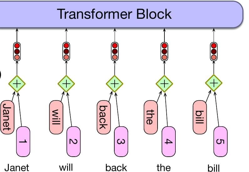
Before the first Transformer block, text must become token IDs. The slides show a byte-pair-encoding (BPE) example: “Thanks for all the” is mapped to illustrative IDs , then each ID selects a row from embedding matrix . These exact numbers are only an example; a different tokenizer or vocabulary would assign different IDs and might split the phrase into a different number of pieces.

BPE starts with small units and repeatedly merges frequent neighboring units according to a learned merge list. In use, the resulting vocabulary contains a mixture of whole words, word pieces, punctuation, and other text fragments. That is why “one token” does not always mean “one English word.” The vocabulary size controls the number of embedding rows and output scores; the sequence length counts tokenizer units, not printed words. A rare name may use several tokens, which changes both context length and prediction cost.

Once tokenized, the row lookup is simple: . The embeddings themselves are parameters trained with the rest of the network. Even if a model is later fine-tuned on a downstream task, its tokenization and embedding rows are the starting point for every input.

Position Is Part of Meaning

If we supply only token embeddings, self-attention has no inherent notion of first, second, or last. With no position signal and no order-dependent mask, permuting input rows permutes output rows in the same way: the operation is permutation equivariant, not invariant. The slide calls it “invariant,” but equivariant is the more precise term for sequence outputs. It means the model cannot distinguish order purely from the token multiset. “Dog bites person” and “Person bites dog” would contain the same token IDs; order must enter somewhere.

The simplest solution is an absolute position table and an input sum

There is one -dimensional position vector for every supported index. The slide’s shorthand is not the shape of the full vector table; the position vectors must match the token-embedding width to be added. can be learned, or positions can be encoded with fixed sinusoidal functions. In the original Transformer, with even/odd feature indices and ,

The different frequencies supply multiple scales of position. This is not the only modern choice, but it is the one pictured in the original architecture. The position signal is added, not appended, in the slide’s example, so the model width stays .

Each input row is a token vector plus its position vector. Course slide 59.

The Language-Model Head

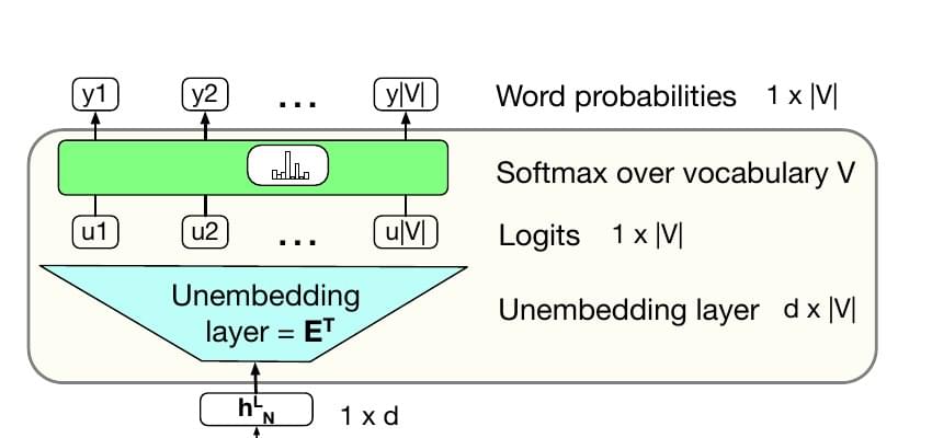
After the final block, a decoder-only language model has a contextual vector at each position. To predict a token, it needs one score for each vocabulary entry. An unembedding matrix and optional bias produce logits and probabilities:

Logits are unnormalized scores; softmax turns them into a distribution. If , there are 50,000 logits for that position—not 50,000 generated words. During training, cross-entropy rewards high probability on the actual next token. At inference, decoding chooses or samples one token and appends it to the context.

The head maps a -wide state to vocabulary scores, then softmax. Course slide 60.

Weight Tying

Input embeddings have shape ; the output projection has shape . Weight tying sets when shapes and vocabulary usage allow it. The same learned token geometry is then used both to enter the model and to score output candidates. This can also act as a useful constraint on learning.

Without tying, the input and output matrices contain about parameters; with tying, about . Thus tying halves these two matrices’ combined parameter count. It does not automatically halve all parameters in the Transformer, because attention and feed-forward layers may account for much of the total. The slide’s “50%” statement is best interpreted at the embedding/unembedding pair, not as a universal whole-model saving.

From Scores to a Continuation

Put the pieces together for a prompt: tokenize it, add token and position vectors, pass them through causal blocks, take the final position’s logits, choose one next token, append it, and repeat. At each generation step the prefix length grows. A key–value cache can retain previously computed attention keys and values so the model need not recompute every old state from scratch, but the next output token still depends on the one just chosen.

The slide’s flow from token IDs to embeddings to layers to unembedding to softmax is therefore a concrete generative algorithm. The probability distribution is the model’s output for one step; the text continuation is produced by repeatedly using that output. Greedy decoding, sampling, temperature, and other decoding policies can turn the same logits into different continuations, but those policies are separate from the architecture covered here.

The Transformer Block

Residual Paths

The original Transformer diagram repeatedly says “Add & Norm.” The add is a residual connection: a sublayer’s output is combined with the representation it received. For a sublayer ,

This gives information and gradients a direct path through deep stacks. It does not mean the network is “skipping learning”; can still make large or subtle changes. It means every sublayer learns an update to an existing representation, rather than having to rebuild the entire representation from nothing. The addition also requires matching widths, which is why multi-head attention projects its concatenated output back to .

Layer Normalization

Layer normalization operates on one token’s feature vector at a time, not across all tokens in a sentence. For ,

The small prevents division by zero. Learned and can rescale and shift normalized coordinates; normalization does not force every subsequent representation to remain permanently zero-mean and unit-variance. Unlike batch normalization, the calculation does not depend on other examples in the minibatch. That makes it a natural component for variable-length text and token-wise processing.

The slide’s block equation uses a post-norm layout: and . A common alternative is pre-norm, where normalization comes before each sublayer, for example . The distinction affects optimization and should not be silently mixed when copying equations or implementing a model. The lecture’s visual “Add & Norm” corresponds to the original post-norm presentation.

Position-Wise Feed-Forward Network

Attention transfers information between positions. The following feed-forward network transforms the features within each position using the same parameters at every position. A typical two-layer form is

where , , and is a nonlinearity. is often wider than . Without the nonlinearity, two linear maps collapse to one linear map, reducing what the sublayer can express. The operation can be applied independently to every token row, which is why it is also described as a position-wise network or MLP.

This division of labor is worth remembering: attention asks which other positions should influence me? The FFN asks how should I transform the resulting feature mixture? Residual paths preserve an ongoing stream through both. Repeating these blocks lets later attention act on increasingly contextual representations.

One Complete Block

In the lecture’s post-norm notation, a self-attention block can be summarized as

For a decoder, uses a causal mask; in an encoder, it normally sees the full input. An original encoder–decoder decoder also inserts a cross-attention sublayer between self-attention and the FFN. We have now accounted for the token and position inputs, Q/K/V projections, attention weights, multiple heads, residual additions, normalization, position-wise nonlinearity, and the output vocabulary head. The remaining architectural change in this lecture is to replace the dense FFN with conditionally selected experts.

Mixture of Experts

Dense Capacity, Sparse Computation

In a dense FFN, every token activates the same FFN parameters. If we simply make that FFN much larger, both parameter count and per-token computation rise. A mixture-of-experts (MoE) layer tries to separate capacity from computation: maintain several FFNs, called experts, but ask a router to select only a small subset for each token. The attention layer can remain ordinary dense attention while the FFN sublayer becomes an MoE sublayer.

Dense computation uses every branch; sparse computation activates only selected branches for an input. Course slide 68.

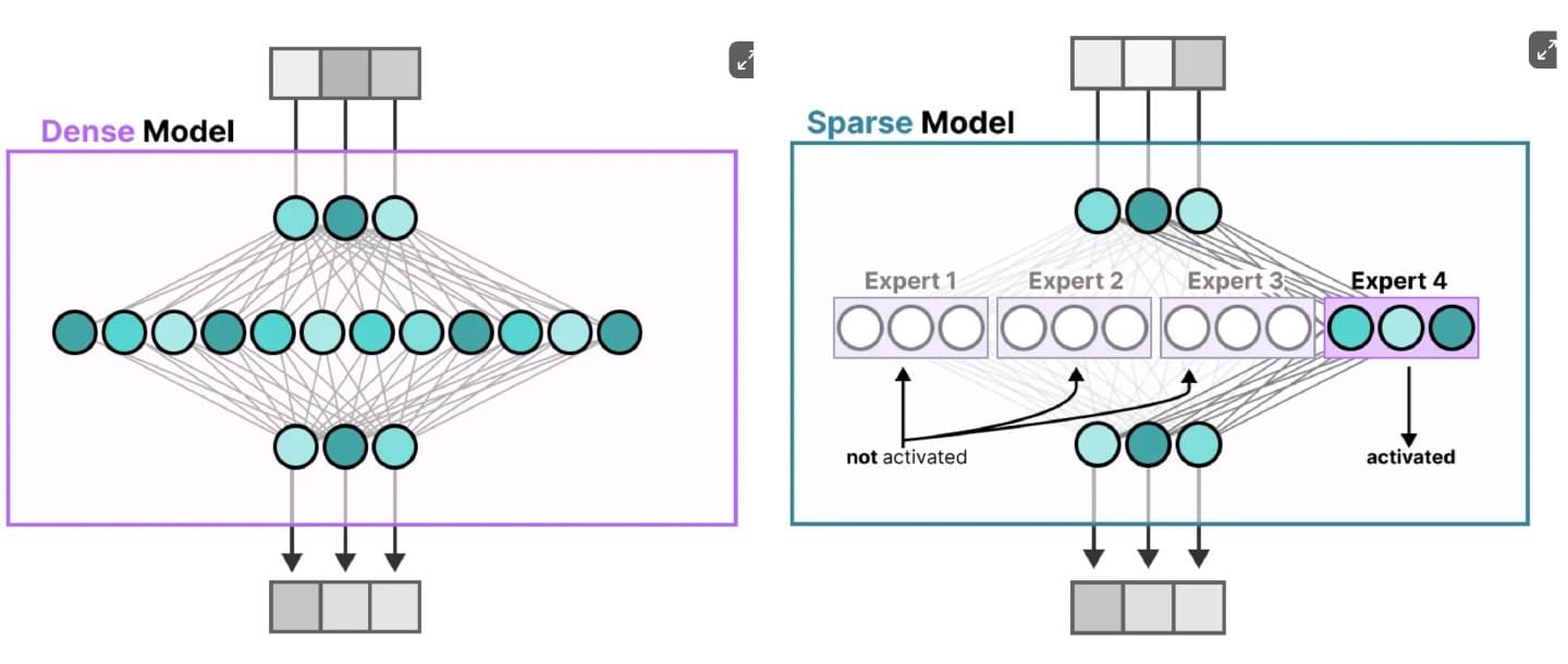
Suppose there are experts , each mapping a token vector to another vector of model width. A router computes scores and normalized weights . If the chosen set has experts, a simple output is

where are the selected weights, optionally renormalized over . The precise normalization varies by implementation. The lecture’s one-expert picture is a top-1 case; other designs choose top-2 or more. The router is trained jointly with the model, so its choices can change as the representation changes.

Different Tokens, Different Paths

The slides show a sentence whose tokens choose different experts, and later passes in which the selected routes change. Do not read the expert labels as fixed human professions. “Words,” “conjunctions,” or “numbers” are an intuitive illustration; actual experts learn whatever division of work improves the training objective, and their specialization may be partial. Routing is usually per token and per MoE layer. The same word in another sentence can arrive with a different hidden vector and select another route; the next layer can route it differently again.

An MoE decoder replaces the dense FFN sublayer with routed expert FFNs while retaining attention and residual paths. Course slide 73.

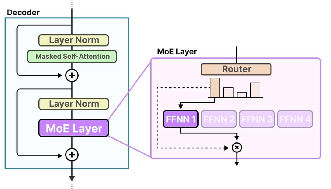
For example, with eight experts and top-2 routing, a token runs two expert networks instead of all eight. That is a reduction in expert arithmetic relative to evaluating all experts, not a promise that the entire model uses one quarter of the FLOPs. Attention, embeddings, routing itself, and other layers still cost work. Nor does a bigger MoE necessarily fit on one device: all expert parameters must be stored somewhere.

Routing Is a Systems Problem

Sparse activation creates new engineering costs. Tokens selected for an expert may need to travel to another accelerator, then return; this is an all-to-all communication pattern. If nearly every token chooses the same expert, that expert becomes overloaded while others sit idle. Systems often impose capacity limits, balancing losses, or other routing controls so the work is spread more evenly. A capacity limit can force some tokens onto alternate routes or cause an overflow policy to drop an expert contribution; implementation details matter.

This is where the previous blog’s systems theme reappears. An MoE can add many parameters without proportional per-token expert computation, but its wall-clock speed depends on routing balance, network bandwidth, expert batch size, and memory placement. The dense versus sparse MoE slide is therefore not a blanket “sparse is better” verdict. Sparse models exchange some regular, local matrix work for conditional work and communication. Use them when that trade-off improves quality and efficiency at the target scale.

Three Architecture Families

Encoder-Only: Understand an Available Input

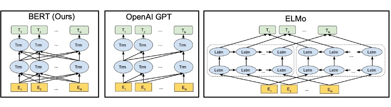
An encoder-only Transformer uses bidirectional self-attention over an input that is fully available. Every position can use evidence on both its left and right, making it a strong foundation for sentence classification, sentence-pair classification, named-entity recognition, sequence tagging, and extracting contextual features. BERT, RoBERTa, ALBERT, and DeBERTa are examples named in the slides. A model can reduce token states to one sentence vector, or keep one output vector per token for tagging.

“Cannot generate text” on the lecture slide is useful shorthand but too absolute. A standard BERT-style encoder is not directly trained for left-to-right free-form generation; that is the relevant architectural distinction. One can design other generation procedures around encoders, but simply asking a bidirectional classifier to continue a prompt is not the model’s ordinary use.

Encoder–Decoder: Transform One Sequence into Another

The original Transformer has a bidirectional encoder for a source and a causal decoder for a target. The decoder uses cross-attention to read source information. This fits translation, summarization, and other conditional generation: the input can be completely read, while output is produced one token at a time. T5 and BART are later examples. Image captioning can follow the same abstract pattern when a suitable image encoder supplies representations to a text decoder; the encoder is then not necessarily a text Transformer.

Decoder-Only: Continue a Prefix

A decoder-only model stacks causal self-attention blocks and predicts the next token from a prefix. This is the direct architecture for open-ended autoregressive generation. The lecture lists GPT-family models, PaLM, Chinchilla, and LLaMA as examples of this broad category. Product names, released checkpoints, and model families should not be treated as interchangeable, but they share the left-to-right modeling pattern at the level relevant here. A decoder-only model can still solve a classification or question-answering task by generating a label or answer as text.

The pretraining comparison: BERT reads both sides, GPT reads a prefix, and ELMo combines separately trained directional LSTMs. Course slide 79.

Transfer Learning: Features or Fine-Tuning

The lecture lists question answering, text generation, summarization, named-entity recognition, and key–value extraction as downstream tasks. There are two broad ways to reuse a pretrained model. A feature-based method freezes some or all of the pretrained network and feeds its hidden representations into another model. A fine-tuning method updates pretrained parameters—often with a small task-specific head—using labeled task data. Prompting a generative model is another way to specify a task at inference time, but it is not identical to parameter fine-tuning.

The best architecture depends on what information is available and what output is required. If the entire document is present and the output is a label for each word, a bidirectional encoder is natural. If a source document is present and the output is a generated summary, an encoder–decoder is natural. If we want a single model to continue arbitrary prompts, a decoder-only model is natural. These are design tendencies, not impossibility theorems. The reason for the choice should always be stated in terms of visibility, training objective, and output format.

BERT in Detail

A Bidirectional Encoder Stack

BERT stands for Bidirectional Encoder Representations from Transformers. It pretrains a stack of Transformer encoder blocks and builds token representations using context on both sides. That differentiates it from early left-to-right GPT, and also from ELMo: ELMo combines separately trained forward and backward language-model states, while BERT’s Transformer layers jointly mix left and right information. Because BERT can see the full input, its pretraining task cannot simply be ordinary next-token prediction with no masking; the target word would be visible in its own input.

The original BERT examples in the lecture use BooksCorpus (about 800 million words) and English Wikipedia (about 2.5 billion words). Two reference configurations show how depth, width, attention heads, and total parameters change together:

Model	Encoder layers	Hidden width	Heads	Parameters
BERT-Base	12	768	12	about 110M
BERT-Large	24	1024	16	about 340M

These are historical pretrained configurations, not mandatory settings for every encoder. More layers allow repeated contextual refinement; greater width allows larger token states; more heads alter how each layer can distribute attention. Increasing any of them also changes training memory and compute.

What Enters BERT

The slide’s BERT input is not merely word embeddings. At each position the model adds a token embedding, a segment embedding, and a position embedding. The special token [CLS] begins the sequence and often supplies a representation for sequence-level classification. [SEP] separates segments or ends a segment. In a sentence pair, segment A and segment B can receive different segment embeddings. BERT’s WordPiece tokenizer can split an unusual word into pieces, illustrated in the slide by play and ##ing.

Token, segment, and position information are added for every input position. Course slide 83.

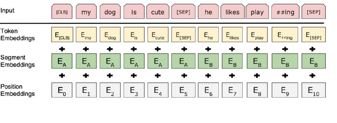
The segment embedding is not an attention mask. It indicates membership in A or B, while padding masks exclude artificial positions. [CLS] is not guaranteed to be a perfect general-purpose sentence embedding out of the box; its usefulness depends on pretraining and the downstream objective.

Masked Tokens and Sentence Pairs

BERT’s masked language modeling selects about 15% of token positions for prediction. At such a position, the model must use surrounding context to identify the original token. In the original recipe, selected tokens are replaced with [MASK] 80% of the time, a random token 10% of the time, and left unchanged 10% of the time; this detail helps reduce the mismatch between pretraining and later inputs, where literal [MASK] tokens are uncommon. The loss is evaluated on the selected positions, not every visible token.

Its second original pretraining task is next sentence prediction (NSP): given segments A and B, classify whether B actually follows A in the source or is a sampled alternative. The [CLS] state provides the pair-level classification signal. The lecture includes both MLM and NSP because they were central to the original BERT design; later variants may change or omit NSP, so do not treat it as a requirement of every encoder model.

These two tasks teach different things. MLM pushes token-level contextual inference. NSP asks the model to use a relationship between two segments. Neither task by itself is the final application; each creates parameters that can be reused and adapted.

Four Downstream Head Patterns

The task diagrams in the slides show four common ways to attach outputs to the same pretrained encoder:

1. Sentence-pair classification: read [CLS] after encoding two segments and predict a relation, such as entailment or paraphrase.
2. Single-sentence classification: read a sequence-level state for sentiment or acceptability.
3. Extractive question answering: encode question and passage together, then predict the start and end positions of an answer span.
4. Token tagging: classify each token state for named entities or other sequence labels.

The same encoder can feed different small task heads; the arrows mark where each task takes its output. Course slide 86.

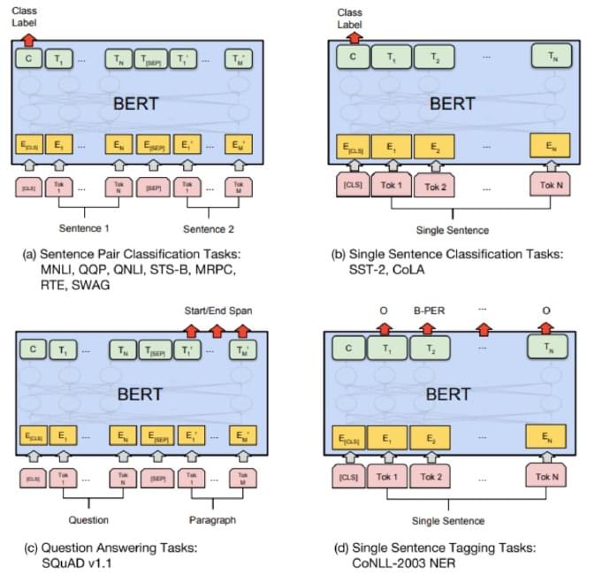
For sentiment analysis, fine-tuning means passing labeled examples through the encoder and training a classification head while updating the chosen BERT parameters. The lecture points to a Colab demonstration of that workflow. The exact dataset and notebook code are not the concept: the reusable pattern is pretrained encoder → task head → supervised fine-tuning → task prediction. For extractive QA, a start/end span head is different from a generative decoder: it selects text already present in the passage.

Which Layer Is the Embedding?

BERT supplies a contextual vector at every layer, not just at the end. If a token passes through 12 encoder blocks, we can use its first layer, last layer, second-to-last layer, a sum of several layers, or a concatenation. The lecture’s NER illustration gives development F1 values of about 91.0 for an early representation, 94.9 for the last hidden layer, 95.5 for a sum over all 12, 95.6 for the second-to-last, 95.9 for a sum of the last four, and 96.1 for a concatenation of the last four. These are results from that particular setup, not universal rankings.

Layer choice changes the feature representation and, in this example, NER F1. Course slide 89.

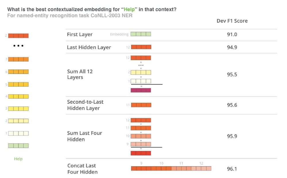
Why might a combination help? Lower and higher layers can preserve different information, and the best representation depends on the task. A concatenation retains more distinctions but increases dimensionality and the downstream head’s parameters; a sum preserves width but blends layers. Select the strategy on held-out data rather than assuming “last layer” is always best. This closes the loop with ELMo’s learned layer mixture: contextualization is not a single immutable lookup table.

GPT, GPT-3, and LLaMA

GPT: Pretrain by Predicting Forward

The early OpenAI GPT model in the slides stacks 12 decoder-only Transformer layers and uses masked self-attention. Its pretraining target is the next token:

At every position, the causal mask ensures the model sees only the prefix. After pretraining, a task can be expressed with an appropriate input format and output head, then fine-tuned. The slide’s transfer-learning diagram lists classification, entailment, similarity, and multiple-choice tasks. They are distinct output formats—one label for a whole input, a relation between two statements, a similarity judgment, or a choice among candidate answers—but the reusable decoder trunk is the common starting point.

Early GPT pretrains a stack of causal decoder blocks and projects hidden states to token scores. Course slide 90.

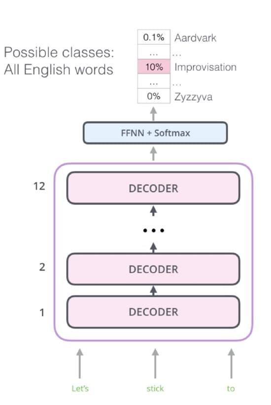
This is an important contrast with BERT. BERT masks selected input tokens and can see both sides of them. GPT never sees future tokens while predicting the next one. A BERT encoder is suited to extracting information from a complete input; a GPT decoder is naturally suited to generating a continuation. Both exploit pretraining, and both can transfer to downstream tasks, but they impose different visibility rules.

GPT-3: A Family, Not One Size

GPT-3 scales the decoder-only approach from 125 million to 175 billion parameters. The slide reproduces a table of eight configurations from the GPT-3 paper . Its columns show that scaling is not “increase parameter count” in isolation: layer count, hidden width, head count, batch size, and learning rate all change. Batch is measured in tokens, not number of documents.

GPT-3 variant	Params	Layers	Width	Heads	Head width	Batch tokens	Learning rate
Small	125M	12	768	12	64	0.5M
Medium	350M	24	1024	16	64	0.5M
Large	760M	24	1536	16	96	0.5M
XL	1.3B	24	2048	24	128	1M
2.7B	2.7B	32	2560	32	80	1M
6.7B	6.7B	32	4096	32	128	2M
13B	13B	40	5140	40	128	2M
175B	175B	96	12288	96	128	3.2M

The 175B row is the model often meant by “GPT-3,” but the other rows matter: a family of controlled sizes lets researchers study how performance changes with scale. The paper also emphasizes few-shot use: examples can be written in the prompt without updating model weights. That is different from the supervised fine-tuning workflow shown for early GPT and BERT. A few-shot prompt may elicit a task behavior, but its examples consume context and do not permanently change parameters.

Data Mixtures, Not Just Data Volume

The GPT-3 slide’s second table gives the training mixture. Quantity is available tokens in each source; weight is how often the source is sampled in training; epochs approximates how many passes through that source occur during a 300B-token run. These are different concepts. A small high-weight corpus can be repeated several times, while a huge web corpus may be sampled for less than one full pass.

GPT-3 source	Available tokens	Mixture weight	Approx. epochs
Filtered Common Crawl	410B	60%	0.44
WebText2	19B	22%	2.9
Books1	12B	8%	1.9
Books2	55B	8%	0.43
Wikipedia	3B	3%	3.4

The weights sum to 101% because the displayed percentages are rounded. The apparent paradox that Wikipedia has very few available tokens but more than three epochs disappears once you distinguish data size from sampling probability. Training data mixture is an architectural-scale design decision: it affects language quality, domain coverage, repetition, and possible memorization. “More web text” alone does not tell us how often books or encyclopedic writing were actually encountered.

LLaMA as Another Decoder Family

The lecture ends with the original LLaMA paper , another decoder-only model family. Its slide table shows four sizes. The labels are approximate public size names; the table’s parameter counts are more specific.

LLaMA variant	Parameters	Width	Heads	Layers	Learning rate	Batch tokens	Training tokens
7B	6.7B	4096	32	32		4M	1.0T
13B	13.0B	5120	40	40		4M	1.0T
33B	32.5B	6656	52	60		4M	1.4T
65B	65.2B	8192	64	80		4M	1.4T

Its displayed pretraining mixture has CommonCrawl 67% and C4 15%, with GitHub, Wikipedia, and books at 4.5% each, arXiv at 2.5%, and StackExchange at 2%. The slide also reports approximate source sizes and passes: CommonCrawl 3.3 TB/1.10 epochs, C4 783 GB/1.06, GitHub 328 GB/0.64, Wikipedia 83 GB/2.45, books 85 GB/2.23, arXiv 92 GB/1.06, and StackExchange 78 GB/1.03. These values describe that historical training mixture, not every later model called “LLaMA.”

The connection to GPT-3 is more informative than a winner/loser comparison. Both are decoder-only, but they choose different model sizes, token budgets, and data mixtures. The table invites three separate questions: How much capacity does the model have? How many training tokens does it see? What distribution do those tokens come from? A parameter count alone answers only the first.

The Thread to Keep

This lecture begins with a fixed word vector and ends with a large generative model, but there is one continuous story. A static embedding gives a token a starting point; a contextual model changes that token’s representation according to its sentence. Attention makes contextual selection explicit through queries, keys, values, and weighted sums. Matrix computation and masking make that selection efficient and respect each architecture’s information boundary. Stacked blocks add residual stability, normalization, and within-token nonlinear processing. MoE changes which FFN parameters are active. Finally, the pretraining objective—bidirectional masking or left-to-right prediction—determines what an encoder or decoder is naturally prepared to do.

When you look at a new model diagram, ask in this order: What are its input units? Which positions can each position see? What is the attention pattern? What does one block compute? Which parameters activate? What target trained the model? How are its final states turned into the task output? Those questions will tell you more than the model’s name or parameter count.