LLM 1 - Fundamentals of Deep Learning

These notes reorganize Lecture 1 by knowledge, not by slide order. The lecture moves back and forth between statistical learning, hardware, distributed optimization, and benchmarking; here those pieces are connected into one systems story. Every technical topic that appears in the slides is retained, while repeated examples are merged and explained together.
The central idea is simple: a capable model is only one component of a useful AI system. Data, optimization, numerical precision, accelerators, communication, software, evaluation, deployment, and monitoring all shape the final result.
1. Why AI Scaled
Four Drivers
The current wave of AI did not come from a single breakthrough. It emerged from the interaction of four forces:
- Algorithms: better architectures, optimization methods, and training recipes.
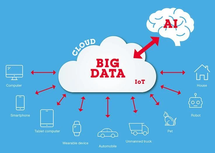
- Data: web, social, mobile, scientific, and IoT sources created datasets at unprecedented scale.
- Compute: GPUs, TPUs, tensor cores, and distributed clusters made large matrix operations practical.
- Applications: useful products generated investment, feedback, and further data.
These forces form a feedback loop. Better compute makes larger experiments possible; better algorithms turn that compute into quality; useful applications produce demand and sometimes new data; revenue and scientific value fund the next generation of infrastructure. Removing any one component slows the loop.
Cloud Shift
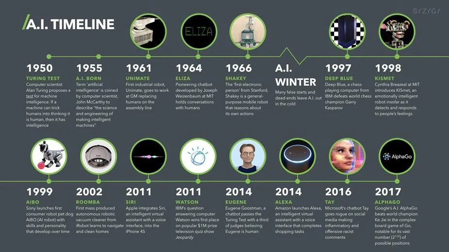
Cloud computing is an important part of this history. Services such as Amazon EC2 and S3, introduced around 2006, separated access to compute and storage from ownership of a physical data center. On-demand resources made it possible to experiment at one scale and train at another.
Elasticity matters because AI demand is uneven. A team may prepare data for days, burst to hundreds of accelerators for training, then serve with a smaller continuously running fleet. Cloud abstractions allow these phases to use different resource shapes, although moving large datasets and reserving scarce accelerators remain significant engineering problems.
AlexNet
AlexNet is a useful historical marker. Its five convolutional and three fully connected layers were trained on GPUs, and it won the ImageNet competition by roughly an 11-percentage-point margin. The lesson was not only that convolutional networks worked; specialized parallel hardware had become a decisive part of model progress.
Its success demonstrated co-design: the network, data, implementation, and available GPU memory were chosen together. This pattern continues in LLMs, where attention kernels, tensor shapes, precision, and parallelism are often adapted to the target hardware.
Foundation Models
Modern language models continue the same pattern at a much larger scale. Training can span hundreds or thousands of accelerators. More parameters increase arithmetic work, while larger datasets increase both compute and I/O. Once a single device can no longer hold or efficiently process the workload, model design becomes inseparable from memory layout, network topology, collective communication, fault recovery, and cost.
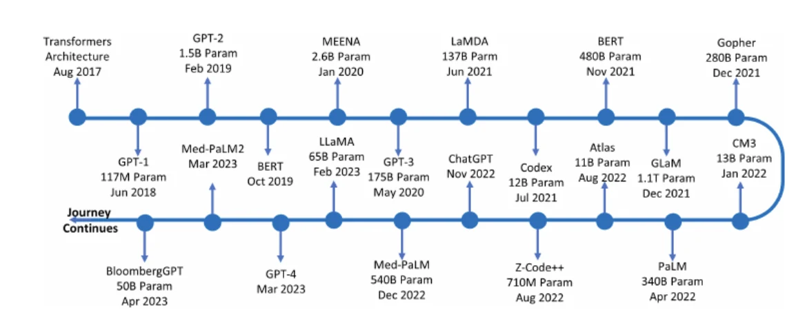
A rapid sequence of model releases—from early large language models to BERT, GPT-family models, LLaMA, Gemini, Claude, and Granite—also changes how systems are built. Organizations may choose a proprietary API, an open model, a domain-adapted model, or a model trained from scratch. Each choice changes data governance, fine-tuning, serving, and evaluation requirements.
The IBM US Open example illustrates a domain system rather than a standalone model. It combines watsonx, Granite models, and watsonx.data with proprietary tennis data to create match reports and commentary. The value comes from grounding a general model in trusted data and integrating it into a reliable workflow.
The example also clarifies why proprietary data can be more defensible than model access alone. Many organizations can call a similar base model; fewer have the same historical records, domain definitions, review process, and product integration.
2. System Stack
Definition
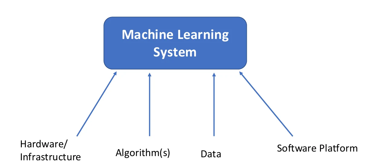
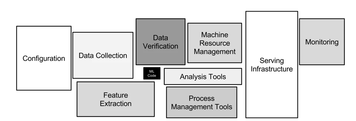
A machine-learning system is a collection of interacting components built to achieve a measurable objective:
The components should not be optimized independently. A model with fewer arithmetic operations may still run slower if its operations have poor kernel support or cause irregular memory access. Likewise, a faster accelerator may sit idle if preprocessing cannot supply batches quickly enough.
Infrastructure and Models
Infrastructure includes CPUs, GPUs or TPUs, device memory, host memory, disks, object storage, and the links within and between machines. Numerical precision is also a systems decision: FP32, FP16, BF16, and quantized formats trade range, accuracy, memory, and throughput.
Algorithms and models determine the required operations, parameter count, activation memory, optimizer state, and communication pattern. Their resource requirements are not fixed in isolation; the same architecture can have very different costs under different batch sizes, precisions, and parallelization strategies.
During training, memory must usually hold more than model parameters: activations needed by backpropagation, gradients, and optimizer states can dominate. An Adam-style optimizer commonly stores multiple auxiliary values per parameter. This is why a model whose weights fit on one GPU may still require sharding for training.
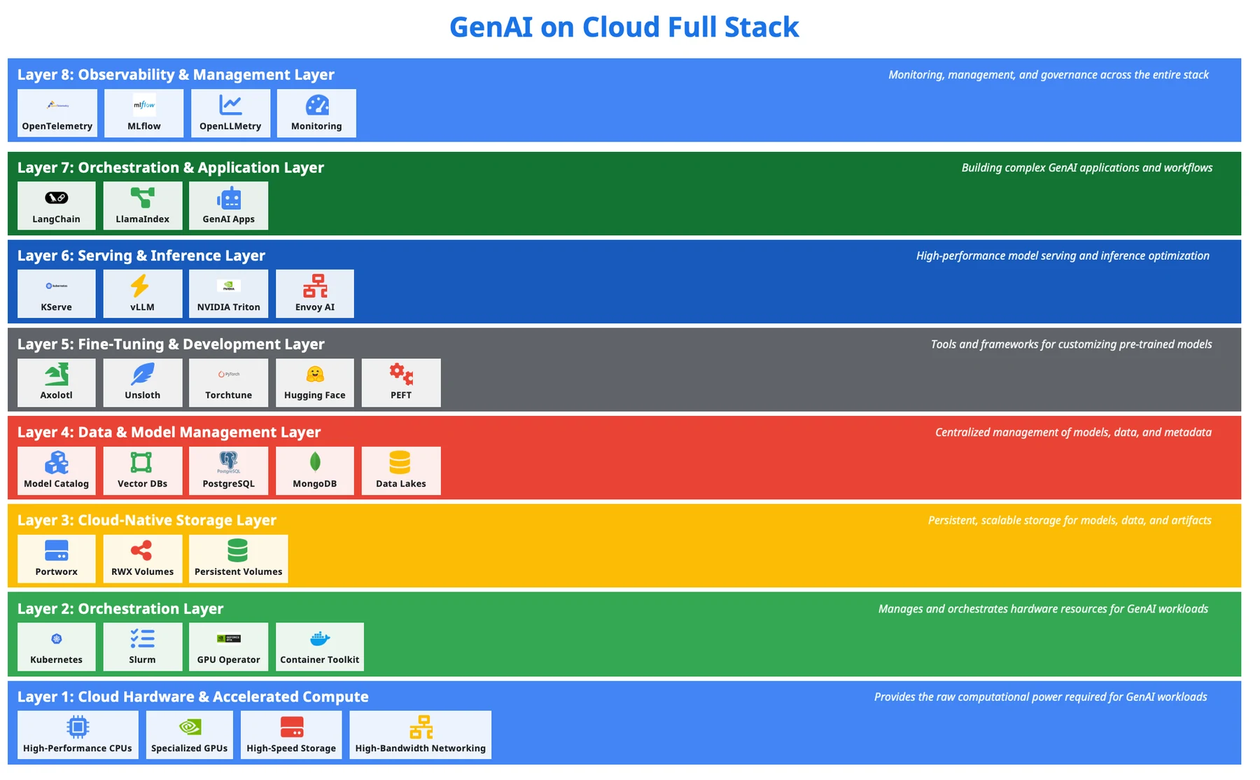
A production generative-AI platform further separates data management, model development, serving, orchestration, and observability into layers.
Data
Data can be text, image, audio, video, time series, graphs, tables, sensor streams, or multimodal mixtures. Its source, representativeness, quality, labeling, access control, storage layout, and movement all matter. A common industry observation is that as much as 80% of project effort can go into preparing data. DataOps practices make ingestion, validation, versioning, transformation, and delivery repeatable.
Data quality sets a ceiling on model quality. Duplicates can cause memorization and benchmark leakage; biased sampling can make performance fail for underrepresented groups; inconsistent labels create irreducible-looking noise; and train/serve skew appears when production preprocessing differs from training. Versioning both raw and transformed data makes these failures diagnosable.
Software and MLOps
Software turns algorithms into an operational pipeline. It includes frameworks and kernels, Docker containers, Kubernetes orchestration, model servers such as TensorFlow Serving, runtimes such as ONNX Runtime, and workflow systems such as Kubeflow. It also includes APIs, logging, CI/CD, and tests for data, infrastructure, models, and production behavior.
Containers package code and dependencies; orchestrators place, restart, and scale workloads; serving runtimes execute models efficiently; workflow systems connect stages and record their inputs and outputs. CI/CD for ML must test not only source code but also schemas, feature distributions, model quality, latency, and compatibility between model and service.
Production Requirements
This is why studying ML systems matters. An algorithm can be correct and still fail because data arrives late, a kernel underutilizes the GPU, workers wait on the network, a dependency cannot be reproduced, or a production distribution drifts away from the training distribution.
Important production properties include:
- Predictability: known latency, throughput, and failure behavior.
- Reproducibility: the same code, data, configuration, and environment can recreate a result.
- Traceability and provenance: a prediction or model version can be connected to its data, code, configuration, and training run.
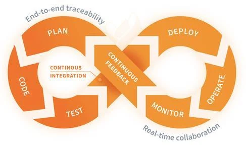
- Automation: deployment, testing, rollback, and retraining do not rely on fragile manual steps.
- Diagnostics and observability: errors and performance regressions can be located quickly.
- Governance and compliance: data and model use can be audited and controlled.
- Scalability and collaboration: teams can share artifacts and workloads without losing consistency.
- Monitoring and management: the system remains useful after initial deployment.
These are also common inhibitors to adoption. A strong notebook result is not yet a maintainable service.
3. Cloud Lifecycle
Service Models
Cloud resources are on demand, pay as you go, and heterogeneous. A workload can rent a CPU machine for preprocessing, a GPU cluster for training, object storage for datasets, and smaller instances for serving. The main service layers are:
- IaaS: raw compute, storage, and networking.
- PaaS: managed application and data platforms.
- SaaS: complete applications delivered as a service.
- MLaaS: managed environments for data preparation, training, tuning, deployment, and monitoring.
Moving upward through these layers reduces the infrastructure a team operates directly, but also reduces control. IaaS allows detailed tuning of drivers, networks, and scheduling; MLaaS can launch experiments quickly but may constrain versions, topology, or observability. The best layer depends on whether customization or operational simplicity is more valuable.
Deployment Models
Deployments may use a public cloud, a private cloud, or a hybrid combination. Managed environments such as IBM Watson Studio, Amazon SageMaker, Azure Machine Learning, and Google Vertex AI reduce setup work, but users still choose resources and control lifecycle decisions. Provisioning, maintenance, monitoring, security, and decommissioning remain part of the cost.
Public clouds offer elasticity and a broad service catalog. Private clouds provide direct control over hardware and sensitive data. Hybrid systems can keep regulated data private while using public resources elsewhere, but they add identity, networking, data-movement, and consistency challenges.
Lifecycle
The model lifecycle is broader than training:
- Preprocess: collect, clean, denoise, deduplicate, debias, label, and split data.
- Engineer representations: construct features or tokenized inputs.
- Train: choose a model, initialize it, optimize parameters, tune hyperparameters, synthesize data when appropriate, and apply regularization.
- Harden: test robustness, adversarial behavior, security, safety, and edge cases.
- Serve: package the model, compress or prune it when useful, select batching and hardware, and expose an interface.
- Monitor: measure response time, failures, resource use, quality, and data or concept drift.
- Learn continuously: retrain, adapt, or replace the model when monitored evidence justifies it.
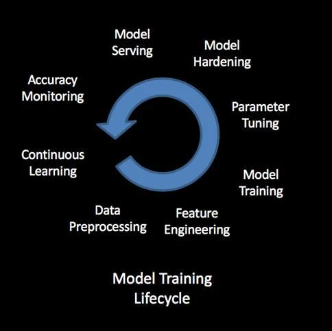
Hardening deserves special attention. Average test accuracy does not reveal sensitivity to adversarial inputs, prompt injection, rare subgroups, corrupted data, or unsafe generations. Hardening defines threat models, evaluates likely failures, and introduces defenses before serving.
Continuous learning should not mean blindly training on recent traffic. Feedback can be delayed, biased, manipulated, or affected by the model’s own prior decisions. A safe loop validates new data, compares candidate and current models, preserves rollback, and monitors post-deployment drift.
Bottlenecks
Each phase has a different bottleneck. Preprocessing may be limited by storage and I/O; training by arithmetic, memory, and communication; serving by memory capacity, memory bandwidth, latency, or concurrency. A lifecycle view prevents local optimizations—such as increasing raw training throughput—from being mistaken for end-to-end improvement.
Amdahl’s-law intuition applies: accelerating one stage has little impact when another dominates total time. End-to-end profiling should separate input time, host-to-device transfer, forward and backward compute, synchronization, checkpointing, validation, and serving queue delay.
4. Generalization
Regression Setup
Supervised learning begins with examples
where
For linear regression,
The residual is
RSS and MSE measure sample prediction error.
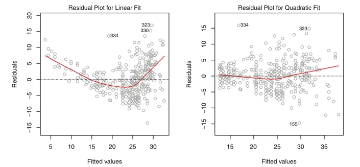
The goal is not to minimize training loss at any cost. It is to predict well on unseen samples from the target distribution.
Linear regression is simple enough to expose the key ideas without hiding them inside a neural network. The feature vector may contain raw variables or a feature map such as
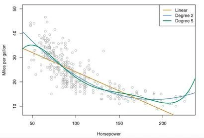
Underfit and Overfit
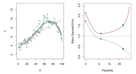
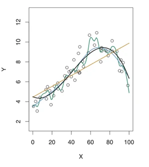
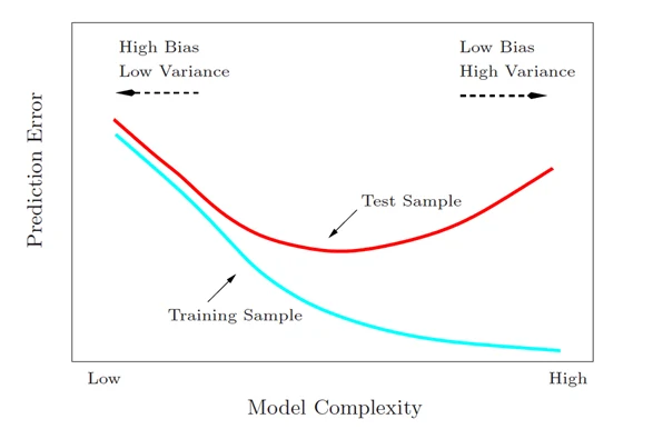
A model underfits when its assumptions or capacity are too restrictive: both training and test errors remain high. It overfits when it models peculiarities of the training sample: training error is low, but test error is much higher. Their difference is the generalization gap.
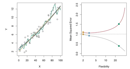
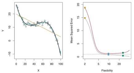
Model complexity can mean polynomial degree, tree depth, feature count, parameter count, or the effective flexibility created by weak regularization. Training error normally cannot increase when a model family becomes strictly more flexible, because the larger family can reproduce the smaller solution. Test error need not follow that monotonic pattern.
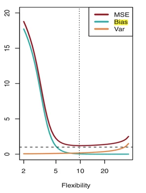
When the true relationship has moderate curvature, test MSE first falls and then rises once the model starts following sample noise.
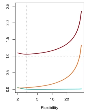
For a more complex target, the best point shifts toward a more flexible model, but the U-shaped test-error pattern remains.
A single fitted curve shows the same problem: an overly flexible line bends toward individual samples instead of the population trend.
Bias and Variance
To formalize the effect of the training sample, imagine repeatedly drawing datasets
from the same population, training a model
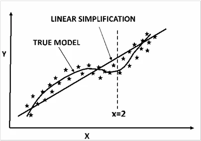
The bias at
The variance measures sensitivity to the sampled training set:
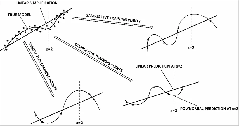
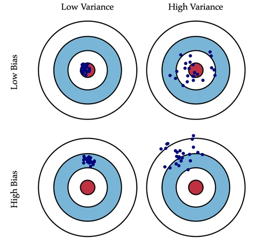
Bias is not simply “the model made an error once.” It is a systematic error visible after averaging over possible training sets. Variance is not observation noise; it is variation in the fitted model caused by which finite sample was observed.
Error Decomposition
If observations contain irreducible noise
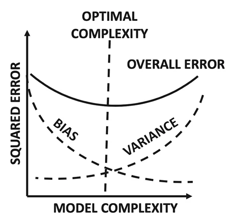
This equation separates three remedies. Reduce squared bias by choosing a more appropriate representation or model. Reduce variance through more data, stronger regularization, ensembling, or lower effective capacity. Irreducible noise cannot be removed by a better predictor unless new information makes the target more predictable.
In a low-noise setting, the test-MSE minimum occurs where falling squared bias and rising variance balance.
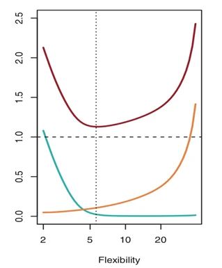
Adding irreducible noise lifts the error floor without changing the basic trade-off.
Putting every component on one graph makes the decomposition operational: test MSE is their sum.
The polynomial interpolation example in the slides makes variance visible. Multiple datasets contain only five sampled points. A sufficiently high-order polynomial can pass through every point, producing low training bias, yet tiny changes in those five observations lead to wildly different curves elsewhere. More expressive models often reduce bias while increasing variance. Neural networks are generally low-bias, high-capacity models, so data volume and regularization are crucial.
Practical Diagnosis
More data usually reduces variance because any one sample has less influence. It does not necessarily fix high bias caused by a wrong representation or overly constrained model. Increasing capacity may reduce bias, but can worsen variance. Generalization is therefore an empirical balance among model family, data, regularization, and optimization.
Learning curves help diagnose the regime. If training and validation errors are both high and close, suspect bias. If training error is low but validation error is much higher, suspect variance or distribution mismatch. If validation performance is strong but production performance falls, inspect dataset shift and pipeline skew rather than automatically enlarging the model.
5. Regularization
Penalized Objective
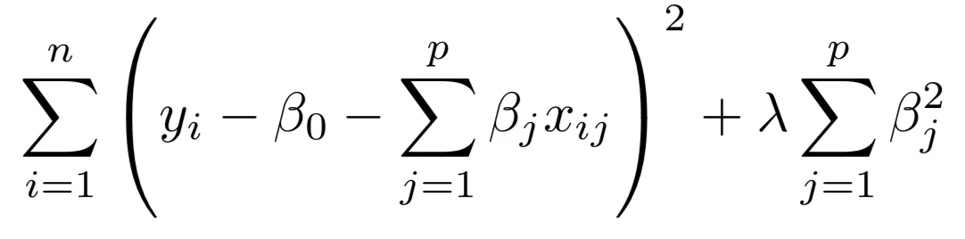
Regularization changes the learning problem so that fitting the data is not the only preference. For data loss
where
This objective encodes a preference among solutions that explain the training data. From a Bayesian view, the penalty resembles a prior over parameters; from an optimization view, it reshapes the loss surface; from a generalization view, it limits effective flexibility.
L1 and L2
Two standard choices are
For least-squares regression, ridge (
As
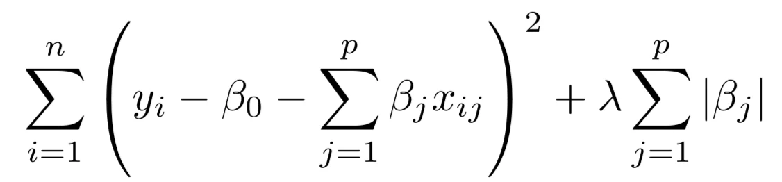
Lasso (
The corners of the
Other Methods
Other forms include:
- adding noise to inputs, activations, gradients, or weights;
- dropout, which randomly removes units during training;
- data augmentation, which creates label-preserving variations;
- early stopping based on validation performance;
- architectural constraints and parameter sharing.
Dropout trains many randomly thinned subnetworks that share parameters, then uses the full network with appropriate scaling at inference. Data augmentation injects domain knowledge by declaring transformations—such as a small image crop—that should preserve the label. Early stopping uses optimization time itself as a capacity control.
Regularization deliberately trades variance for bias. With
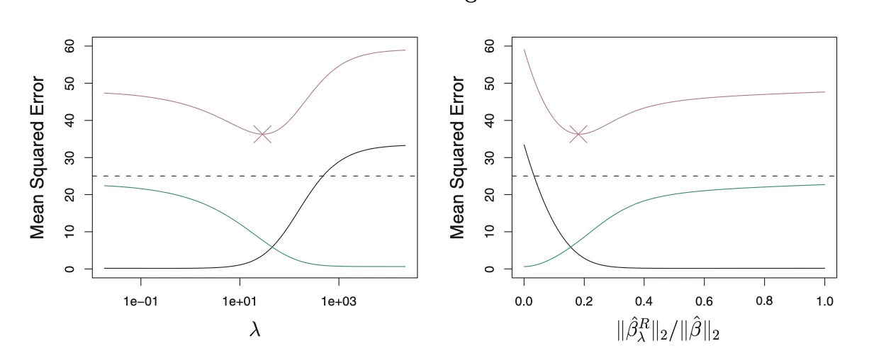
Validation
The validation set is used to choose
Cross-validation is useful when data is scarce, but expensive for deep models. Whatever the protocol, splits must respect the application: time-series data often needs chronological splits, and related users, documents, or scenes may need group-wise separation to avoid leakage.
Implicit Effects
The same logic appears later in distributed training. Small-batch gradient noise can act as implicit regularization and favor flatter solutions, while very large batches may converge to sharper minima that fit training data well but generalize less reliably. System choices can therefore change statistical behavior.
6. Metrics
Confusion Matrix
For binary classification, the confusion matrix contains true positives (
“Positive” names the event of interest, not a morally good outcome. In disease screening, positive may mean disease detected; in fraud detection, it may mean transaction blocked. Metric interpretation begins by defining that event and the cost of each cell.
Core Rates
The core measures are
Two related rates shown in the slides are
Precision conditions on predicted positives: when the system alerts, how often is it right? Recall conditions on actual positives: of the events we needed to find, how many did we find? Specificity asks the analogous question for negatives.
Imbalanced Data
Accuracy can be misleading under class imbalance. A classifier that predicts the 99% majority class every time reaches 99% accuracy while having no ability to detect the minority class. Balanced accuracy gives equal weight to sensitivity and specificity:
The
Always report class prevalence and preferably the full confusion matrix. Precision changes when prevalence changes even if recall and false-positive rate stay fixed. A deployment population with a different base rate can therefore produce a different user experience from the test set.
Threshold Curves
An ROC curve plots true-positive rate against false-positive rate as the decision threshold changes. It describes a family of operating points rather than one fixed classification threshold.
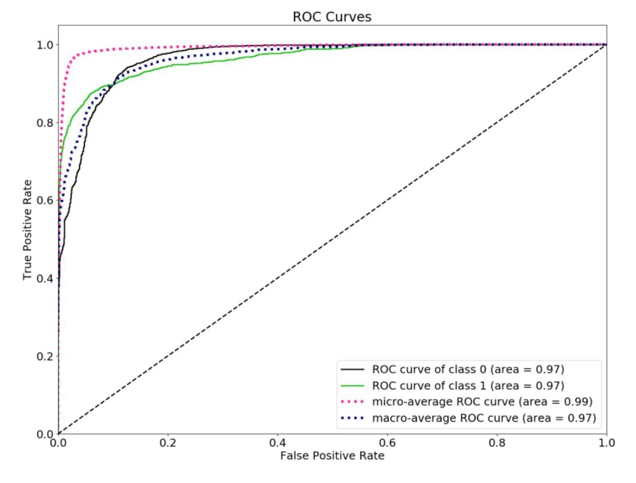
Area under the ROC curve summarizes ranking across thresholds, but it can hide operationally important regions. Precision-recall curves are often more informative when positives are rare. A production threshold should reflect real costs and capacity—for example, how many alerts a review team can inspect.
Model and System
Lecture 1 also separates model quality from system quality. Loss, accuracy, precision, recall, F-score, and ROC describe predictive behavior. Training time, inference latency, throughput, memory, energy, reliability, resource consumption, scaling efficiency, and monetary cost describe practicality. A fair comparison must hold the target quality constant: the fastest run is not useful if it reaches a worse model.
Later course evaluations extend these ideas to language generation. ROUGE, BLEU, and n-gram overlap capture limited aspects of text similarity; GLUE, SuperGLUE, MMLU, BIG-bench, and HELM aggregate task performance; MLPerf, LLMPerf, Hugging Face tooling, and fmperf focus more directly on systems behavior. No single number captures correctness, safety, speed, and cost.
7. Training
Training Loop
Training repeats four conceptual operations:
- A forward pass computes activations and predictions.
- A loss function compares predictions with targets.
- Backpropagation applies partial derivatives and the chain rule to compute gradients.
- An optimizer updates the parameters.
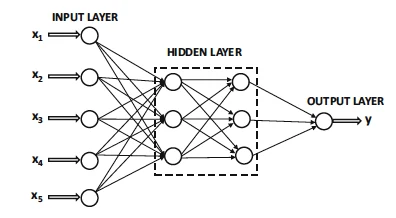
The forward pass stores intermediate activations because the backward pass needs them. For a deep network, these saved activations can consume more memory than the parameters. Backpropagation traverses the computation graph in reverse and accumulates each parameter’s contribution to the loss.
Backpropagation
For a scalar parameter
For a linear unit
For parameters
Gradient Variants
Full-batch gradient descent evaluates the entire dataset before each update. Stochastic gradient descent uses one randomly selected example. Mini-batch SGD uses a subset
This is an approximate gradient, but it is cheaper and maps naturally to dense matrix operations. Randomizing samples prevents ordering effects and makes successive estimates less correlated.
One epoch means processing the full training dataset once, not making one update. With dataset size
Hyperparameters
Training time is jointly determined by compute, memory, and network communication. A step can be slow because matrix operations are expensive, activations and optimizer states exceed device memory, data cannot be delivered quickly enough, or gradients take too long to synchronize.
Important hyperparameters include:
- architecture depth, width, and connectivity;
- activation functions;
- parameter initialization;
- learning rate and its schedule;
- batch size;
- momentum;
- optimizer;
- regularization and weight decay.
They are not learned by ordinary backpropagation, yet they can determine whether training converges.
Momentum smooths noisy directions by carrying a running update velocity. Adaptive optimizers rescale coordinates using gradient statistics. Initialization controls the initial scale of activations and gradients; poor initialization can make signals vanish or explode before useful learning begins.
Training and Inference
The slides use an older hardware example to make scale concrete. AlexNet trained on roughly 2.5 million Places images on a K40 GPU could take about six days. Later P100 and V100 devices increased arithmetic throughput and memory bandwidth substantially.
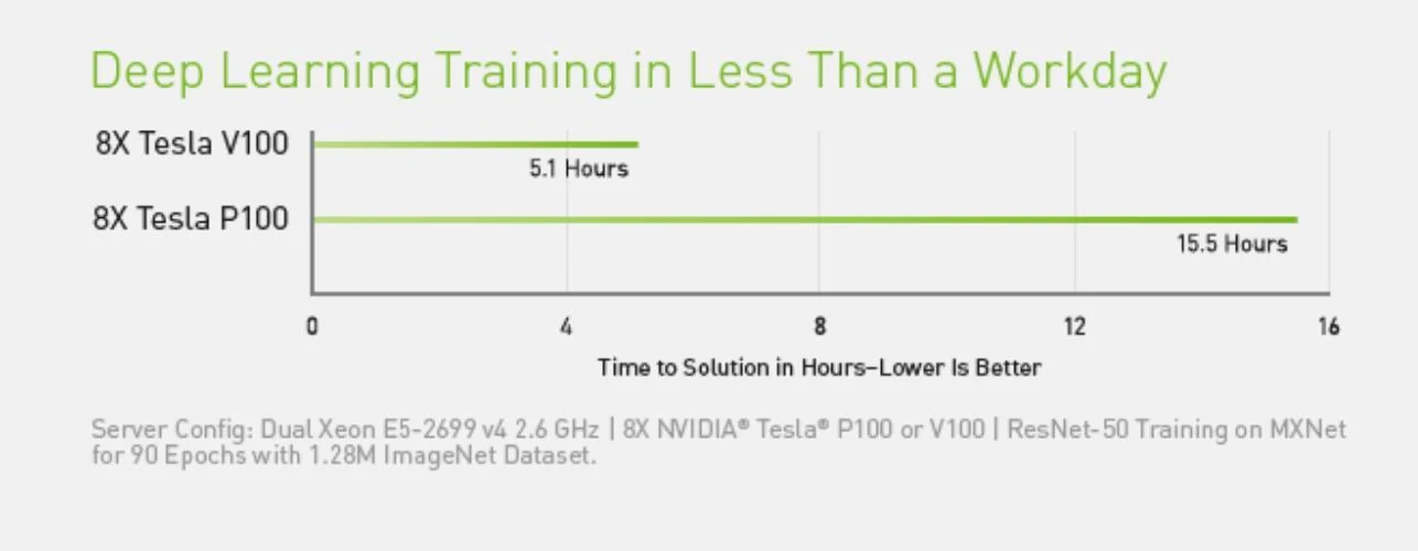
Inference has a different objective. Training emphasizes time to target quality; inference may emphasize queries or tokens per second, tail latency, memory per replica, and cost per request. Optimizing one phase does not automatically optimize the other.
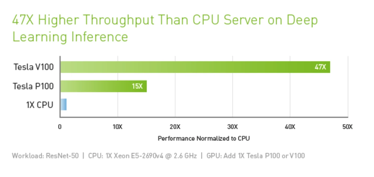
Training needs backward computation and optimizer state; inference does not, but autoregressive generation repeatedly reads model weights and an expanding key-value cache. Training is commonly throughput-oriented, whereas interactive inference must also respect per-request latency and fairness.
8. Batch and Rate
Batch Trade-off
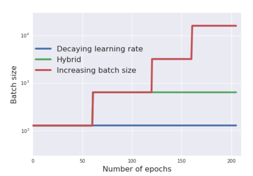
Batch size connects statistics to hardware. Larger batches expose more parallel work, improve accelerator utilization, and provide lower-variance gradient estimates. They also consume more memory, reduce the number of updates per epoch, and may converge to sharp minima with weaker generalization. Smaller batches use less memory and provide noisier updates; that noise can act as implicit regularization and favor flatter solutions.
The historical K40 example has about 12 GB of memory, while common P100 and V100 configurations have about 16 GB. More memory allows a larger batch, but “largest batch that fits” is not the same as “best time to quality.”
The useful quantity is global batch size: local batch per worker multiplied by the number of data-parallel workers, adjusted for gradient accumulation. Accumulation can emulate a larger global batch when memory is limited, although it does not create the same per-step device utilization as a physically larger local batch.
Learning Rate
The learning rate controls update magnitude. Too large a rate can overshoot or diverge; too small a rate wastes steps. A common schedule uses warmup and then decay. Large-batch training often begins with learning-rate scaling, but the relationship must be validated for the model, optimizer, data, and schedule.
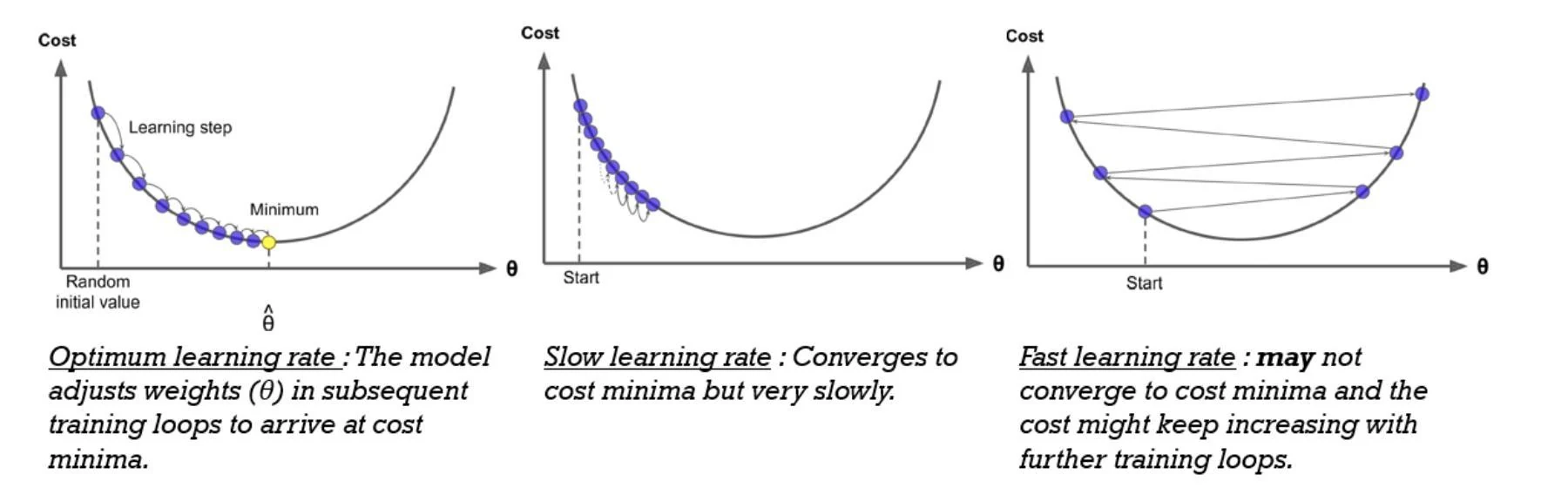
Warmup protects early training when parameters and optimizer statistics are not yet calibrated. Decay allows large exploratory steps early and smaller refining steps later. Step, exponential, cosine, and inverse-square-root schedules express different assumptions about how quickly that transition should occur.
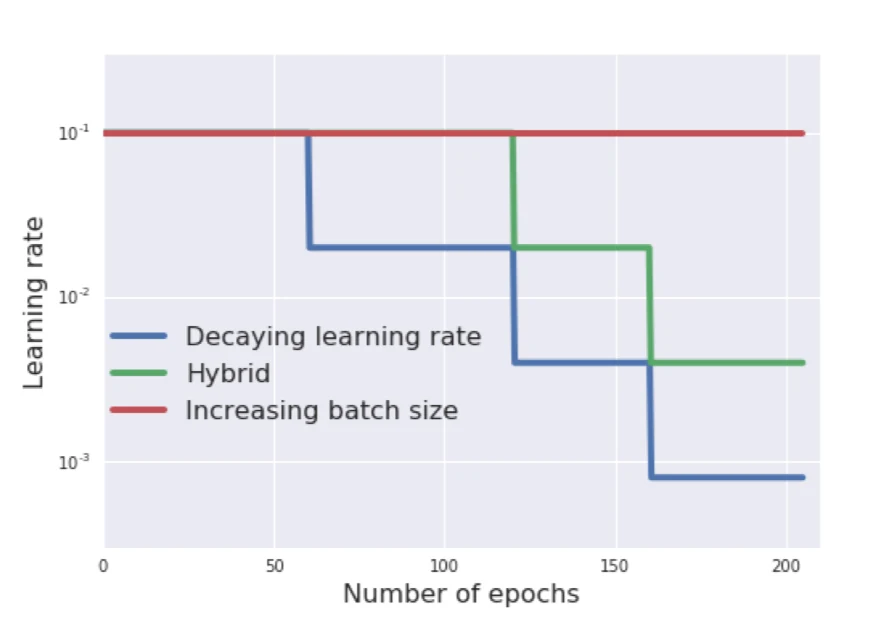
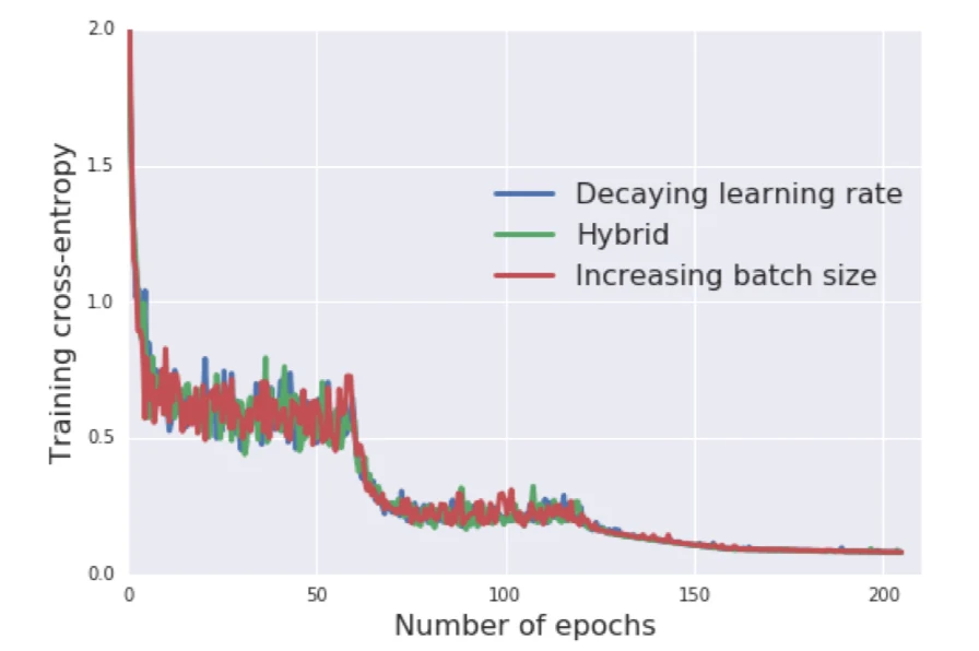
The training-loss curves can remain similar when one method changes the learning rate and another changes batch size, reflecting their shared effect on gradient noise.
Noise Scale
The slides express the relation using a gradient-noise scale:
where
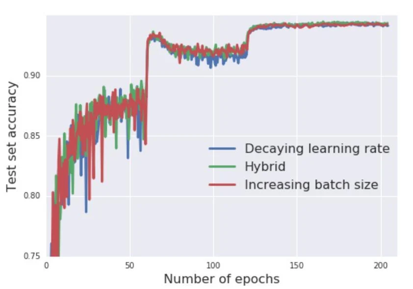
This explains an important equivalence: increasing the batch size reduces gradient noise in a way resembling a decrease in learning rate. To preserve a similar noise scale, an optimal batch can grow roughly in proportion to the learning rate. The relationship is a model, not a universal rule; it is most useful for reasoning about the trade-off.
A larger batch processes the same epoch in fewer optimizer updates. It may have higher examples-per-second but still need careful warmup or more epochs to reach the same accuracy. Report both throughput and final quality.
Batch Normalization
Batch normalization stabilizes the distribution of intermediate activations. For a mini-batch
The small
At inference, batch normalization uses running estimates rather than statistics from the current request. This prevents one prediction from depending on unrelated examples that happen to share a serving batch. The distinction between training and inference mode must be handled correctly when evaluating or exporting a model.
Practical Tuning
A useful tuning order is to find a stable learning-rate range on a manageable batch, increase the batch only while throughput and time-to-quality improve, add warmup when scaling aggressively, and compare runs at the same validation target. Monitor loss spikes, gradient norms, examples per second, memory utilization, and final generalization together.
9. Hardware
Accelerators
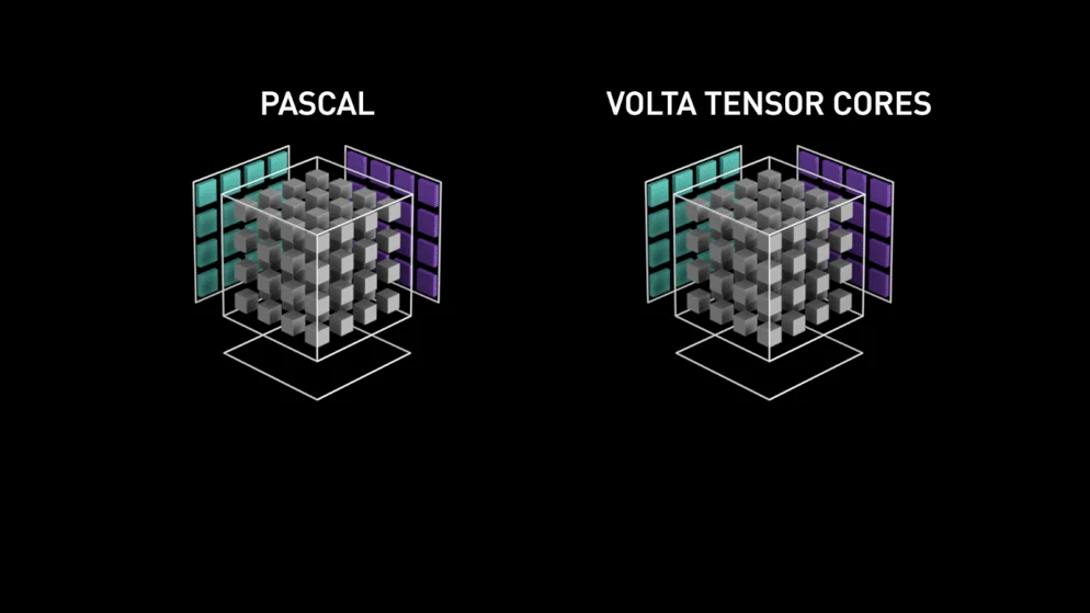
Deep-learning accelerators are effective because training contains large amounts of dense, parallel arithmetic. GPUs provide many execution units and high-bandwidth device memory. TPUs are application-specific integrated circuits designed around tensor operations.
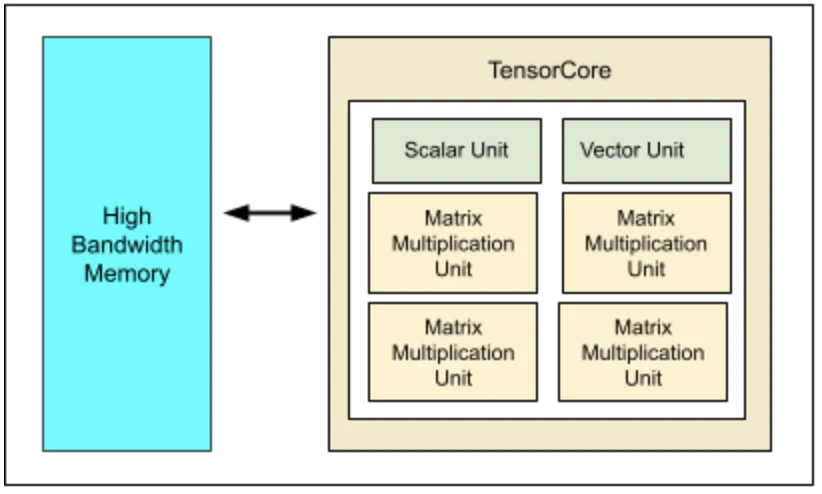
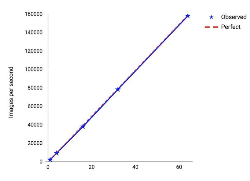
A TPU v5e TensorCore, for example, combines four matrix-multiply units with vector and scalar units. A TPU worker is attached to a host VM, and many workers can form a pod through a dedicated high-speed network. Earlier TPU v2 pod results showed near-linear ResNet scaling over a useful range.
Peak FLOPS describes an upper bound for suitable arithmetic, not application speed. Real utilization depends on tensor dimensions, kernel fusion, memory access, control flow, compiler quality, and whether input and communication stalls leave execution units idle.
Observed TPU throughput can track theoretical scaling when a workload maps well to the architecture.
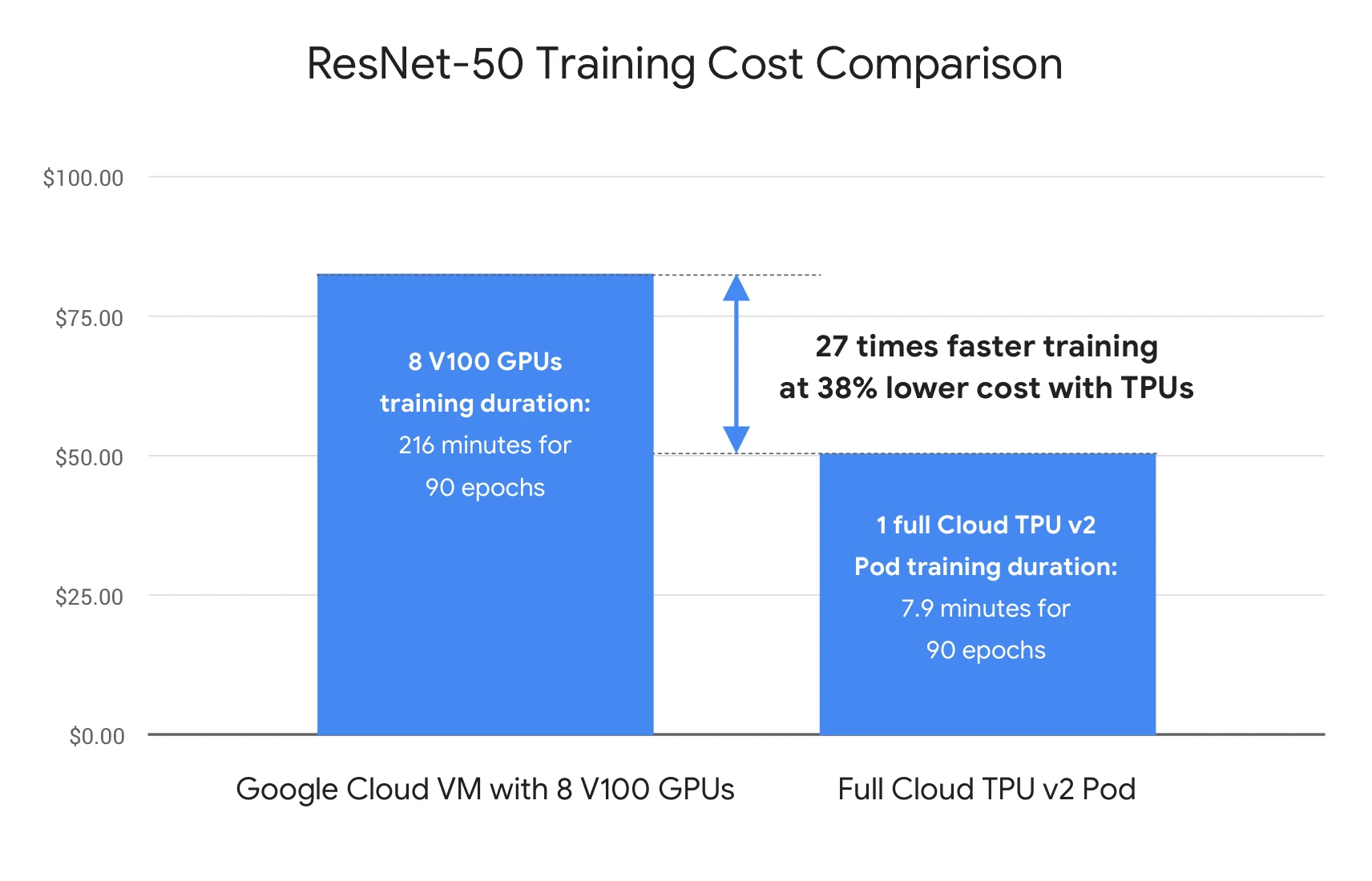
Cost also depends on time: faster hardware can be competitive even at a higher hourly price.
Memory Paths
The device is only one level of a hierarchy:
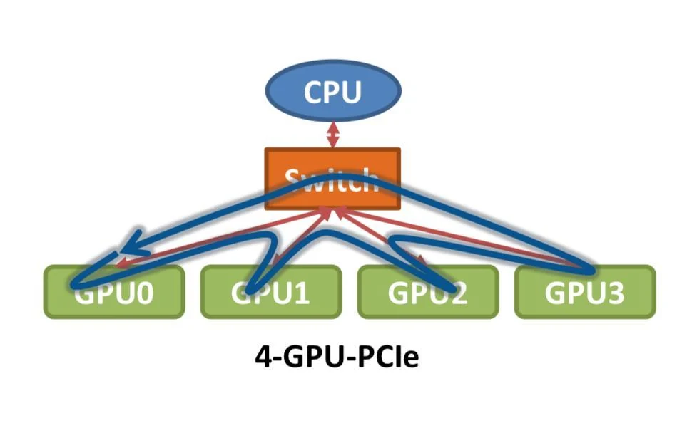
PCIe connects devices and hosts. SMP describes processors sharing a common memory system. Intel QPI is a point-to-point processor interconnect; the slides cite about 25.6 GB/s for a representative link. NVLink provides a much faster GPU-to-GPU path than ordinary host-mediated transfer.
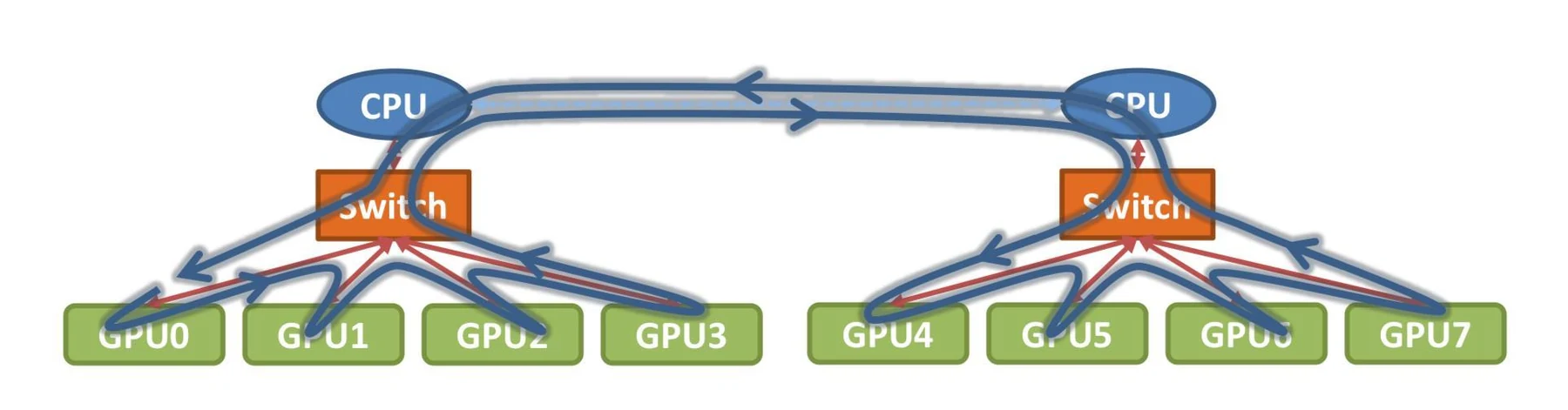
Bandwidth is the amount transferred per second; latency is the fixed delay before useful transfer completes. Large gradient tensors are often bandwidth-bound, while many small messages are latency-bound. Collective algorithms therefore chunk and schedule traffic to use links efficiently.
Network Scale
Representative values in the slides illustrate the orders of magnitude:
| Interconnect | Approx. bandwidth | Approx. latency |
|---|---|---|
| 10 Gigabit Ethernet | 10 Gb/s | 4 μs |
| 40 Gigabit Ethernet | 40 Gb/s | 4 μs |
| InfiniBand EDR | 100 Gb/s | 1 μs |
| NVLink | over 400 Gb/s | 0.1–0.2 μs |
The exact numbers vary by generation and topology, but the principle is stable: moving values between devices can cost much more than operating on values already local to an accelerator.
Effective bandwidth can be far below the link’s advertised rate because of protocol overhead, contention, topology, and incomplete overlap. Profiling should measure application-level collective time rather than infer it from hardware specifications.
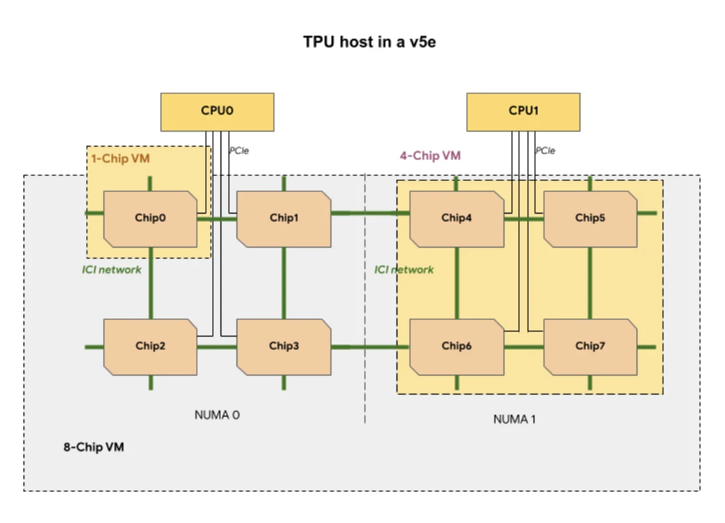
TPU pods also expose topology: chips are grouped under hosts and NUMA domains and connected by a dedicated inter-chip network.
Collectives
NVIDIA’s NCCL library provides topology-aware collective operations:
- broadcast;
- reduce;
- reduce-scatter;
- all-gather;
- all-reduce;
- point-to-point send and receive.
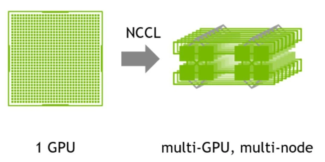
NCCL optimizes paths across PCIe, NVLink, and Mellanox networking. Efficient implementations try to overlap communication with backpropagation, beginning reduction for later-layer gradients while earlier layers are still computing.
Collectives encode a group operation rather than a specific topology. An all-reduce can be implemented with a ring, tree, hierarchical scheme, or a combination selected for message size and machine layout.
Scaling and Precision
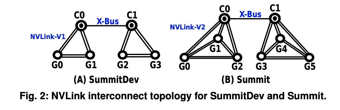
Scaling can be vertical or horizontal. Scale-up places more/faster accelerators inside one tightly connected node; DGX-1 with eight P100s and DGX-2 with sixteen V100s are examples from the slides. Scale-out adds nodes, as in large systems such as Summit or Sierra. Scale-out offers more total resources but makes network behavior and failure management increasingly important.
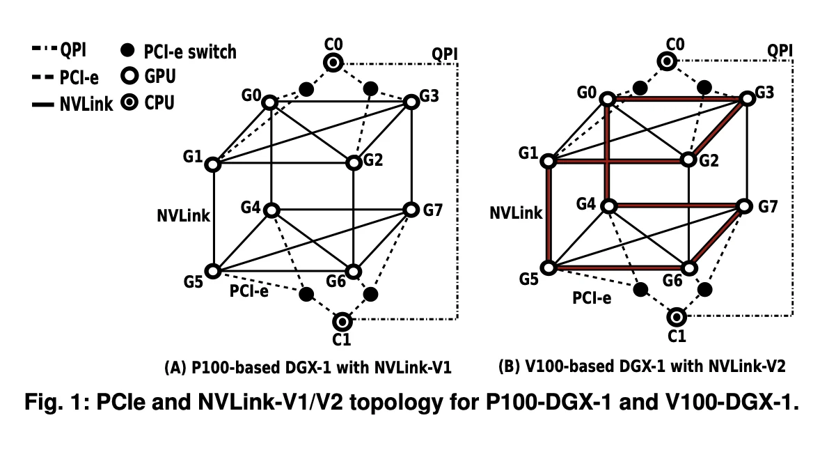
At larger scale, topology becomes a hierarchy of accelerator links, CPU sockets, and inter-node paths.
Lower precision such as FP16 can reduce memory use and increase tensor-core throughput. Mixed-precision training keeps numerically sensitive operations or master weights in higher precision. Precision is therefore both a performance tool and a numerical-stability constraint.
10. Parallelism
Data and Model
When a workload is too large for one device, work can be partitioned by data, model, or both.
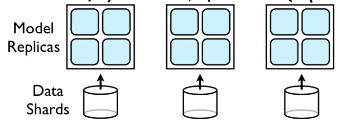
Data parallelism places a complete model replica on each worker and sends each replica a different data shard. Workers compute local gradients, then aggregate them before the next update. This is simple and effective when one model replica fits in device memory.
Model parallelism partitions a model across devices. A simple five-layer network mapped to four learners must transfer activations wherever a layer boundary crosses devices. A poor partition creates excessive communication; locality and physical connectivity matter.
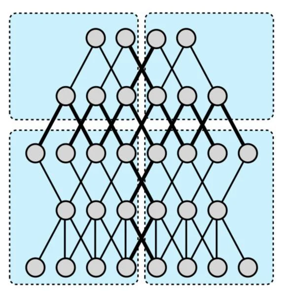
Data parallelism mainly increases compute throughput; model parallelism mainly addresses per-device memory capacity. The first adds gradient synchronization, while the second adds activation and intra-model communication. This difference guides where each dimension should be placed in a cluster.
Pipeline Parallelism
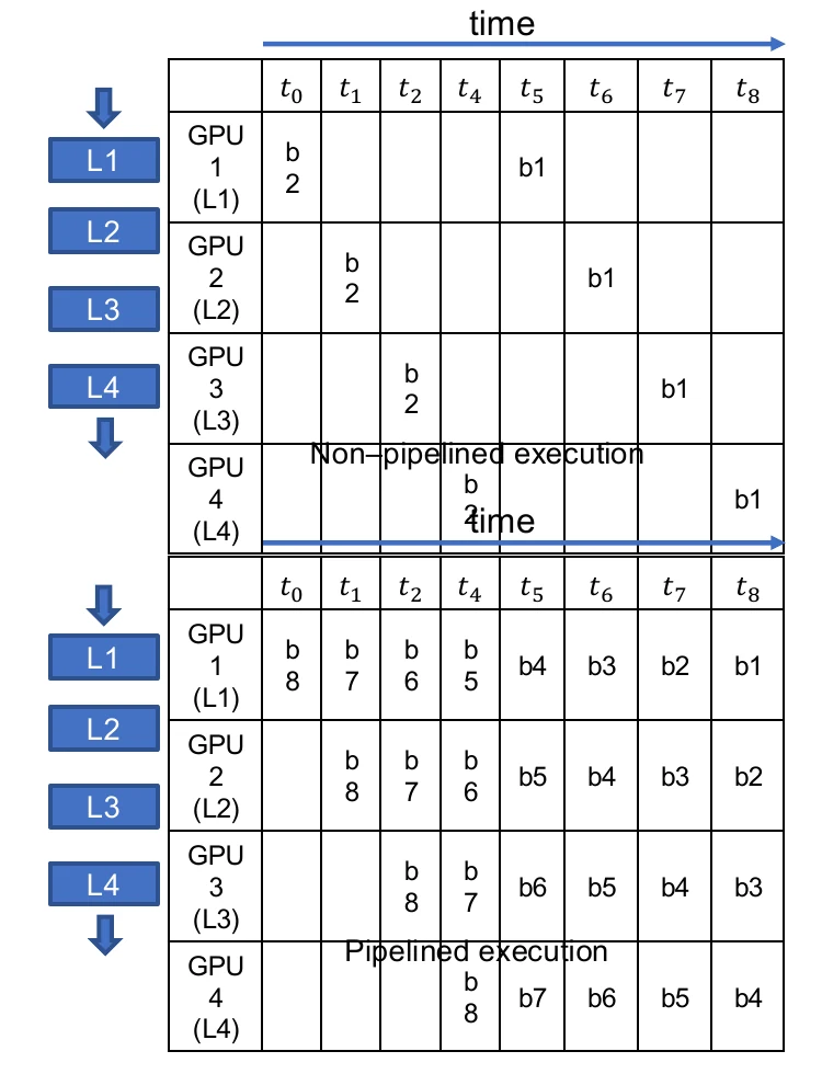
Pipeline parallelism places consecutive layer groups on different devices. Dividing a batch into micro-batches allows stages to operate concurrently, as in GPipe. The activation-memory requirement can scale with the number of in-flight micro-batches, written as
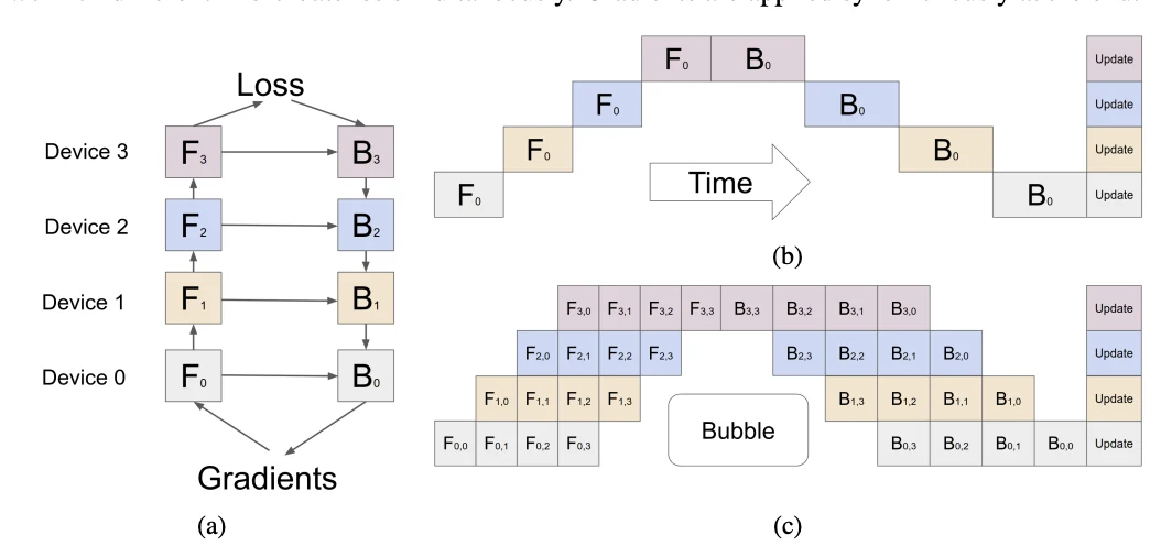
For an ideal pipeline with
More micro-batches reduce the fraction of time spent filling and draining the pipeline, but require more in-flight state and can affect the effective batch. A good partition also balances stage execution time; one slow stage determines pipeline throughput.
Tensor Parallelism
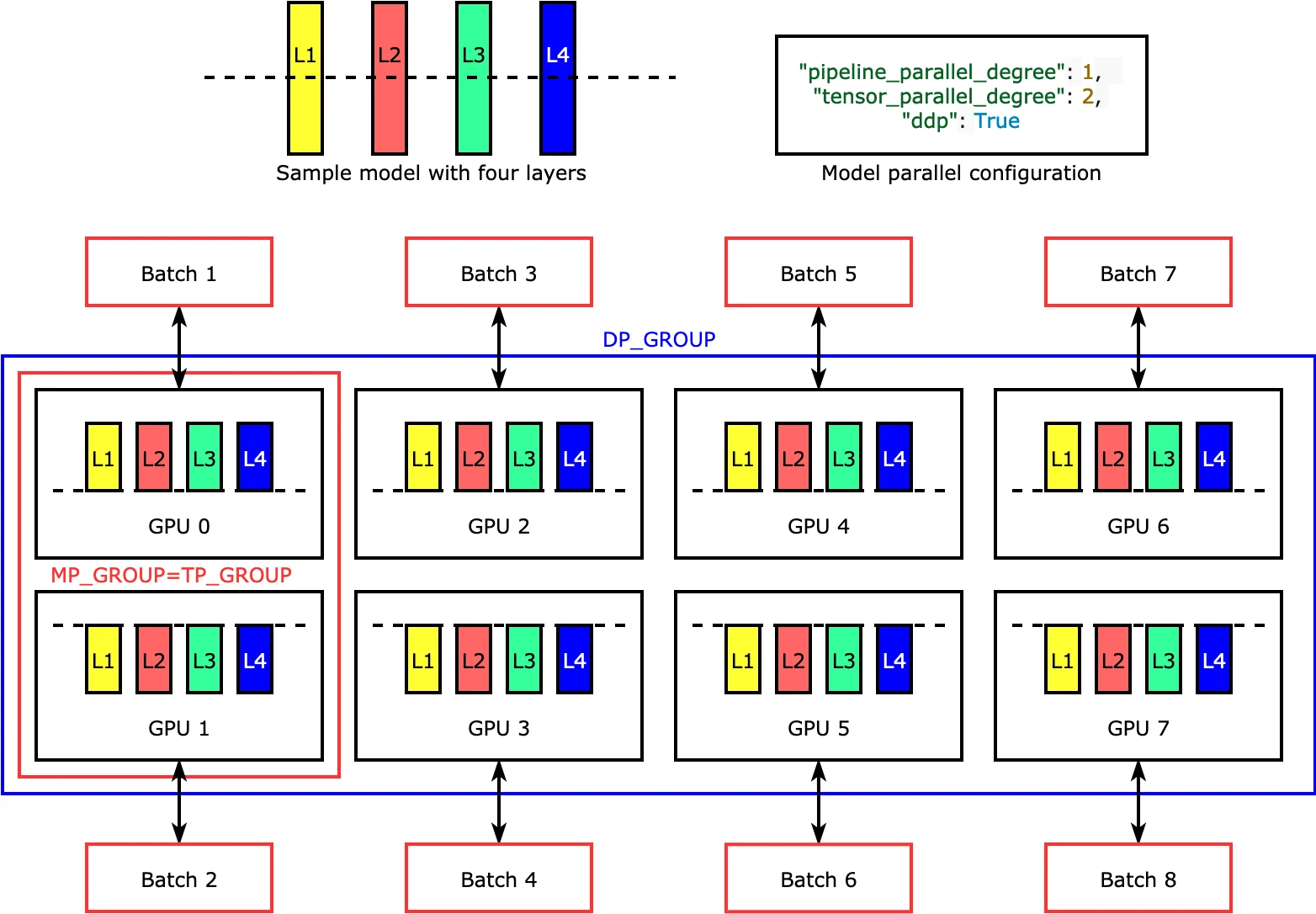
Tensor parallelism partitions individual tensor operations inside a layer. It supports layers too large for one device, but usually requires collectives at every layer, so it is best within a fast local interconnect.
For a matrix multiplication, workers may split rows or columns and then combine partial activations. Because this communication lies on the critical path of every transformer block, tensor-parallel groups are usually kept within an NVLink-connected node when possible.
Hybrid Layout
Modern LLM training combines these methods:
Another example uses two-way tensor parallelism inside each model replica and eight-way data parallelism across replicas. These dimensions form independent process groups: a worker participates in one group for tensor communication and another for replica synchronization.
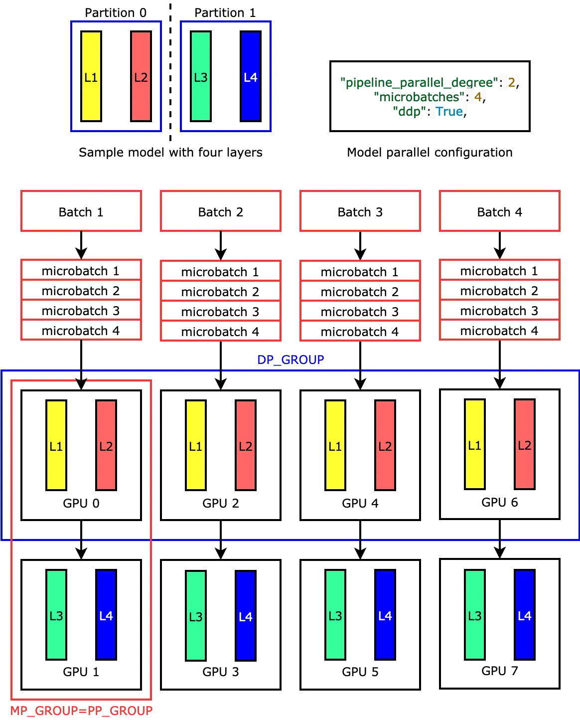
Parallel dimensions multiply. If tensor parallelism is 2, pipeline parallelism is 4, and data parallelism is 8, the job uses
Memory Strategies
Systems such as SageMaker model parallel add:
- pipeline and tensor partitioning;
- optimizer-state sharding;
- activation checkpointing, which recomputes activations instead of storing all of them;
- activation offloading to host memory;
- automated or assisted placement.
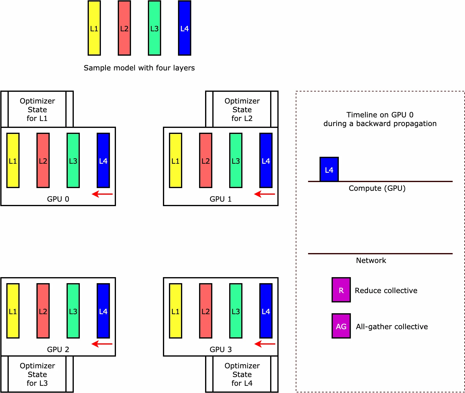
These techniques exchange one resource for another. Sharding saves device memory but increases communication. Checkpointing saves activation memory but increases compute. Offloading extends capacity but uses a slower memory path. A good configuration respects both the model graph and machine topology.
Optimizer sharding underlies methods such as ZeRO and FSDP: instead of keeping every optimizer value, gradient, and parameter replica on every data-parallel rank, selected states are partitioned and gathered when needed. The saving can make a previously impossible model trainable, at the cost of more communication and implementation complexity.
11. Sync and Benchmarks
Synchronous Training
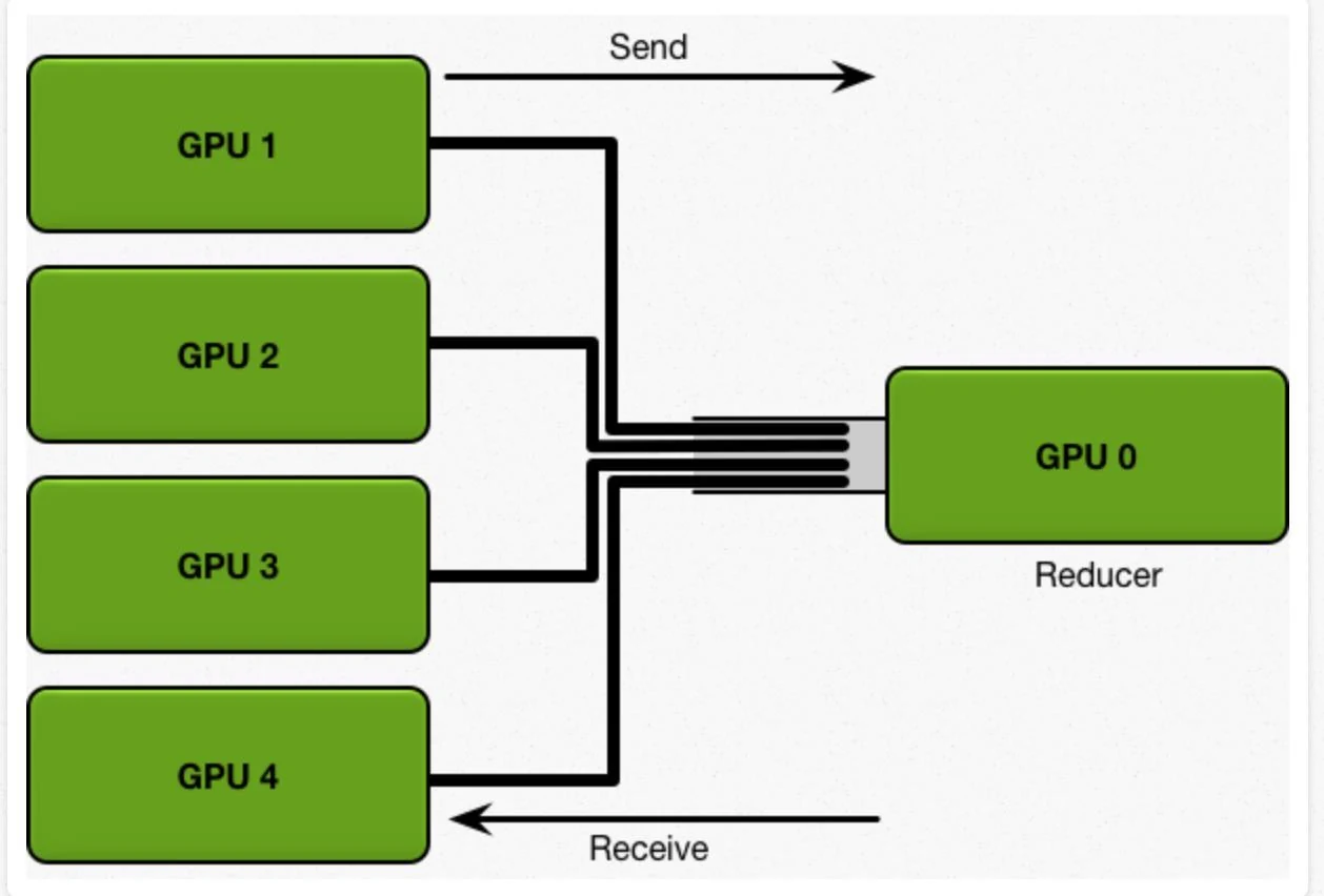
Data-parallel workers must combine gradients. In a parameter-server architecture, workers send gradients to a central server, which aggregates them, updates the model, and distributes new parameters. This is simple, but the server and its network links can become bottlenecks.
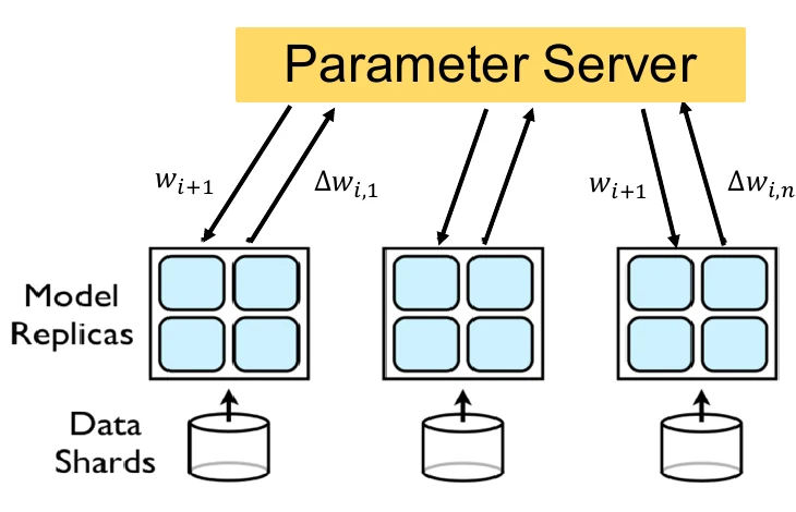
In synchronous SGD, all required workers compute from the same parameter version and the update waits for them. Statistical semantics are clean, but a slow worker delays everyone. Stragglers arise from variation in compute time, data access, network congestion, and shared infrastructure.
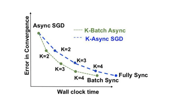
K-synchronous methods update after the first
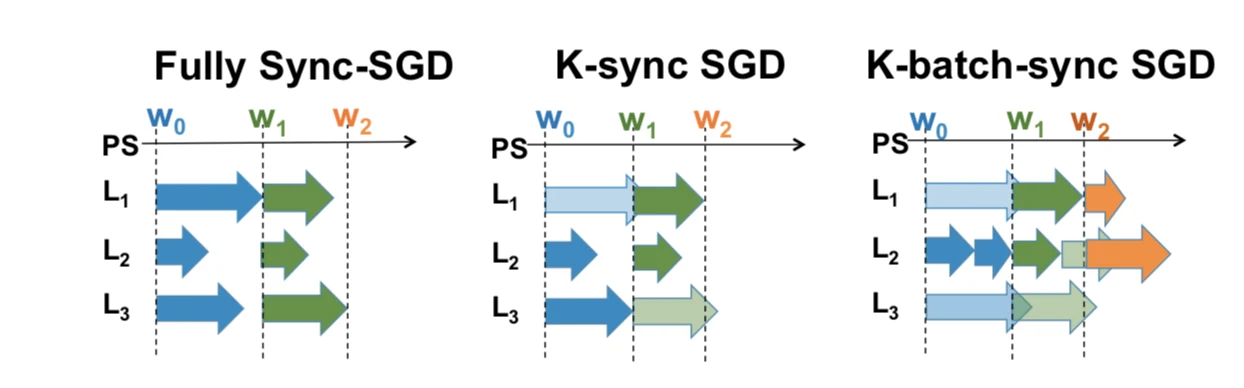
Choosing
Async and Staleness
In asynchronous SGD, a worker sends its result immediately and fetches new parameters without waiting for peers. If it computed using
is stale. K-asynchronous and K-batch asynchronous variants update after a specified number of arriving results, generally without cancelling ongoing work.
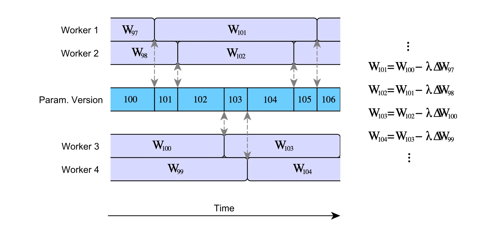
Asynchronous policies differ in whether one arrival,
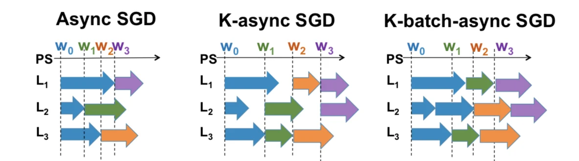
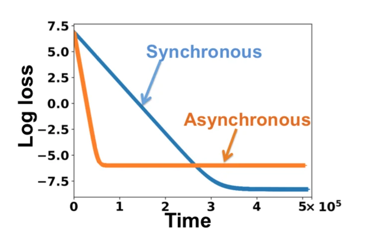
Async execution may reduce error faster per unit of wall-clock time because devices wait less, yet stale gradients can raise the final error floor. A system must compare time to the same target quality, not only seconds per iteration.
Staleness is especially harmful when parameters move rapidly or gradients from different workers point in conflicting directions. Bounded-staleness policies, smaller learning rates, and delay-aware optimization can improve stability, but each changes the original optimization process.
Ring All-Reduce
In synchronous data-parallel training, every worker must obtain the sum or average of all workers’ gradients. A centralized reducer is conceptually simple, but it concentrates all incoming and outgoing traffic on one device.
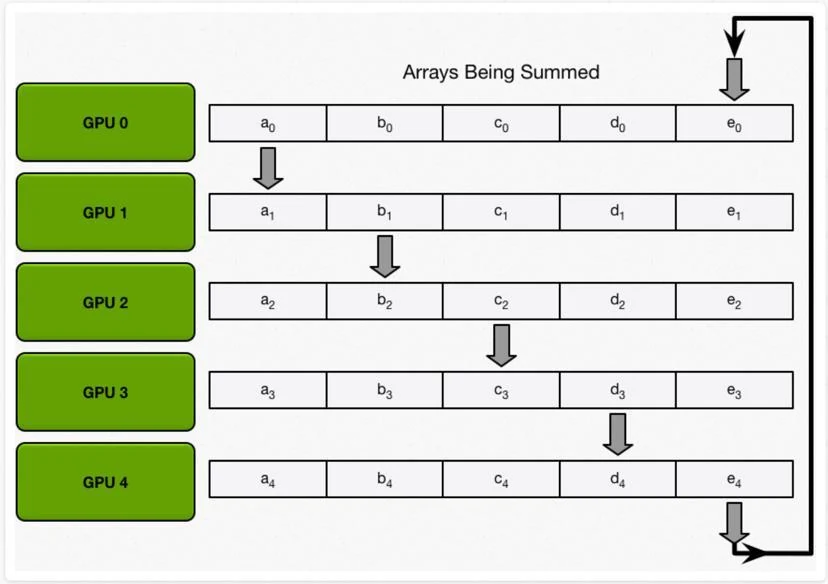
Ring all-reduce removes that central bottleneck by arranging the
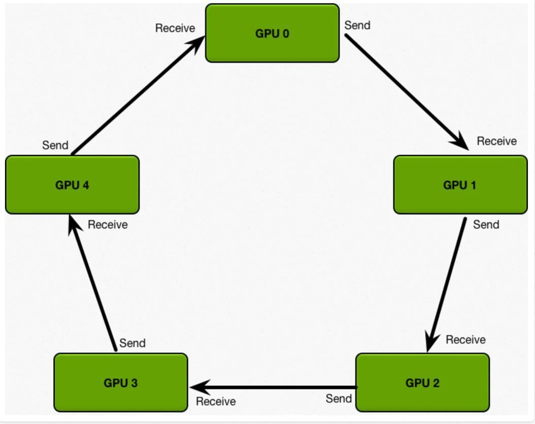
The final objective is unchanged: every process must finish with the same element-wise sum of all local arrays.
To distribute the work, each length-
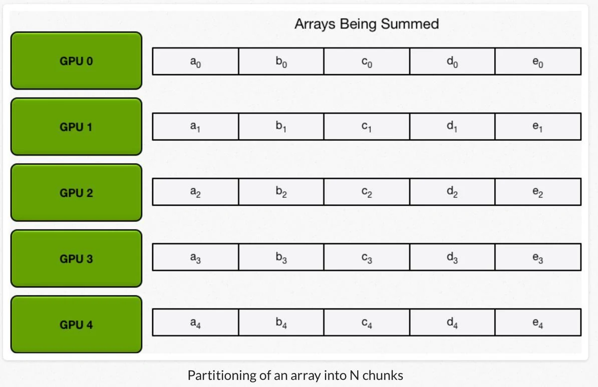
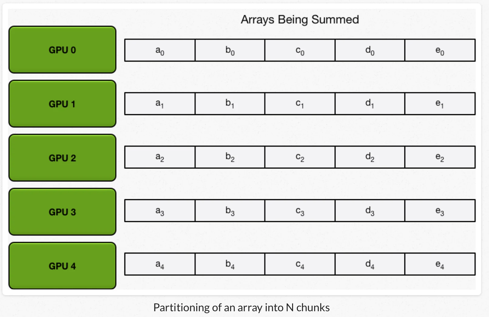
Initially, each GPU owns its own version of every chunk. A chunk must travel around the ring while each receiver adds its corresponding local values.
During reduce-scatter round 1, every GPU sends one chunk clockwise. The receiver immediately reduces that chunk with its local counterpart.
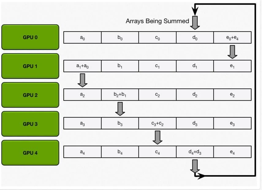
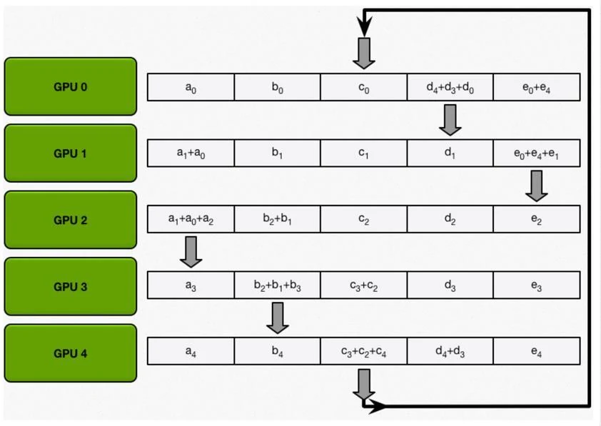
In round 2, the partial sums move to the next neighbor and accumulate another worker’s contribution.
Round 3 repeats the same local operation. No process needs to receive or transmit the entire gradient at once.
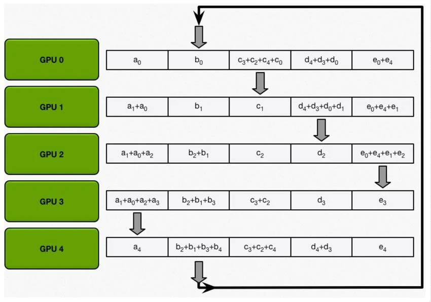
After the final illustrated exchange, every chunk has visited the processes needed to form one complete reduction.
After
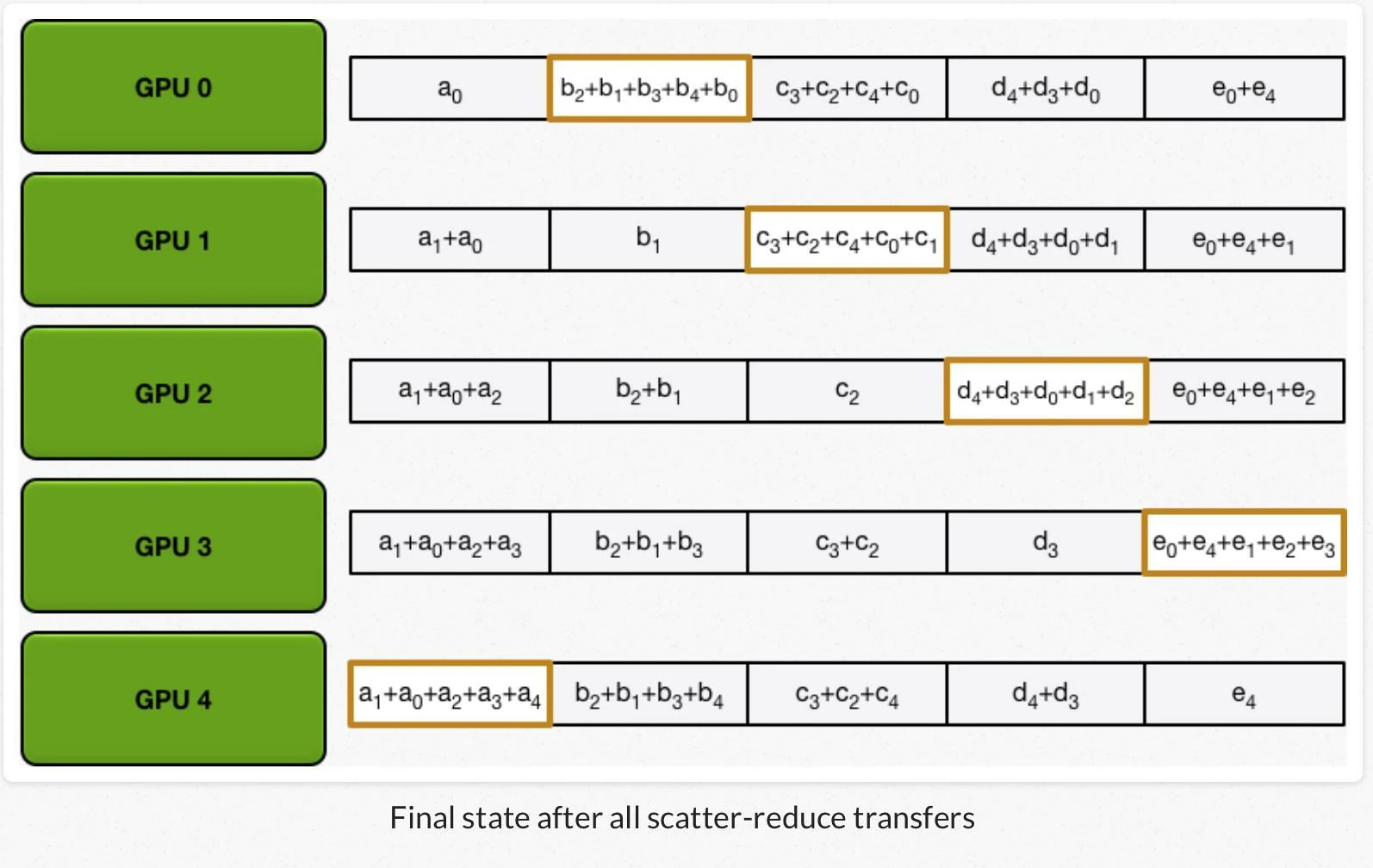
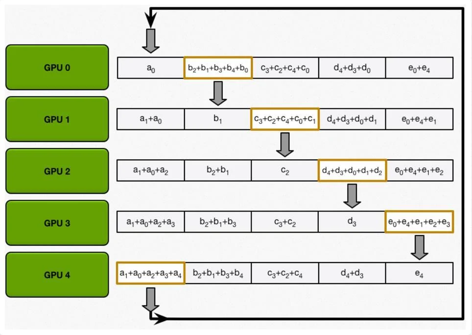
The send/receive schedule is cyclic. For the five-GPU example, the ownership transition can be summarized without preserving a screenshot of the slide’s table:
| GPU | Sends | Receives |
|---|---|---|
| 0 | Chunk 1 | Chunk 0 |
| 1 | Chunk 2 | Chunk 1 |
| 2 | Chunk 3 | Chunk 2 |
| 3 | Chunk 4 | Chunk 3 |
| 4 | Chunk 0 | Chunk 4 |
The all-gather phase now circulates the completed chunks without further addition. In round 1, each owner sends its finished chunk to the next GPU.
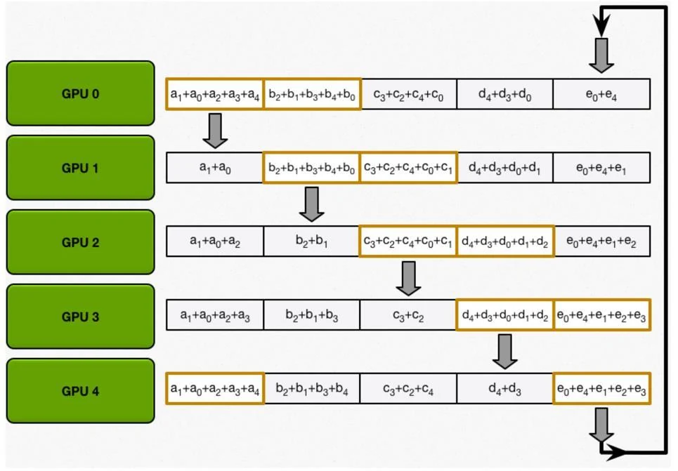
In round 2, each GPU forwards the completed chunk received in the preceding round.
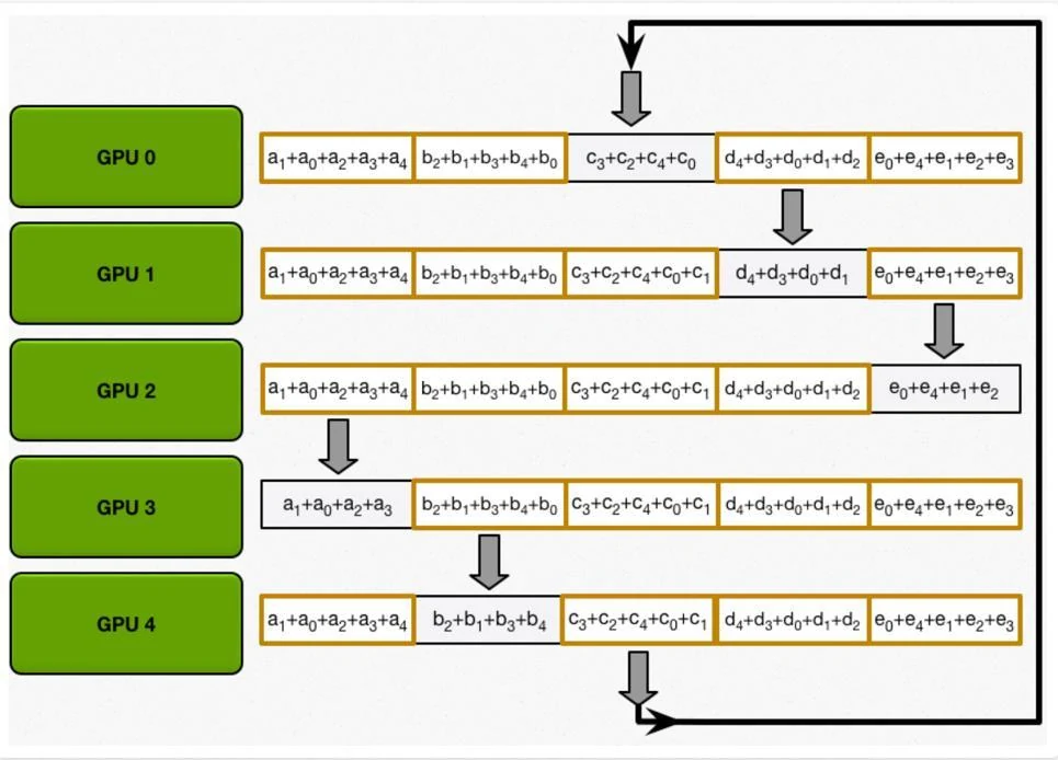
Round 3 continues the circulation; communication is balanced because every GPU sends and receives the same amount per round.
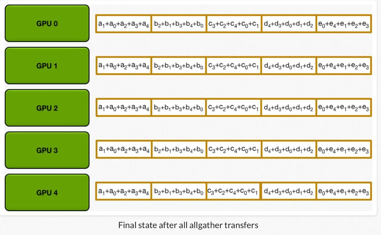
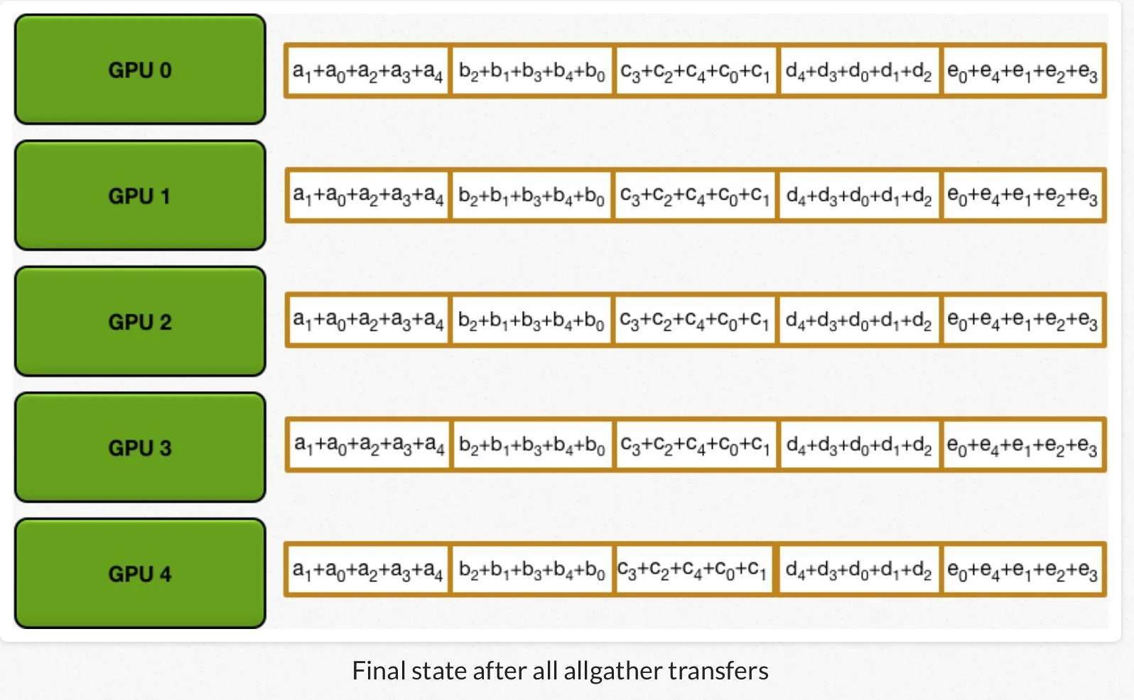
The last exchange delivers the remaining missing chunk to every participant.
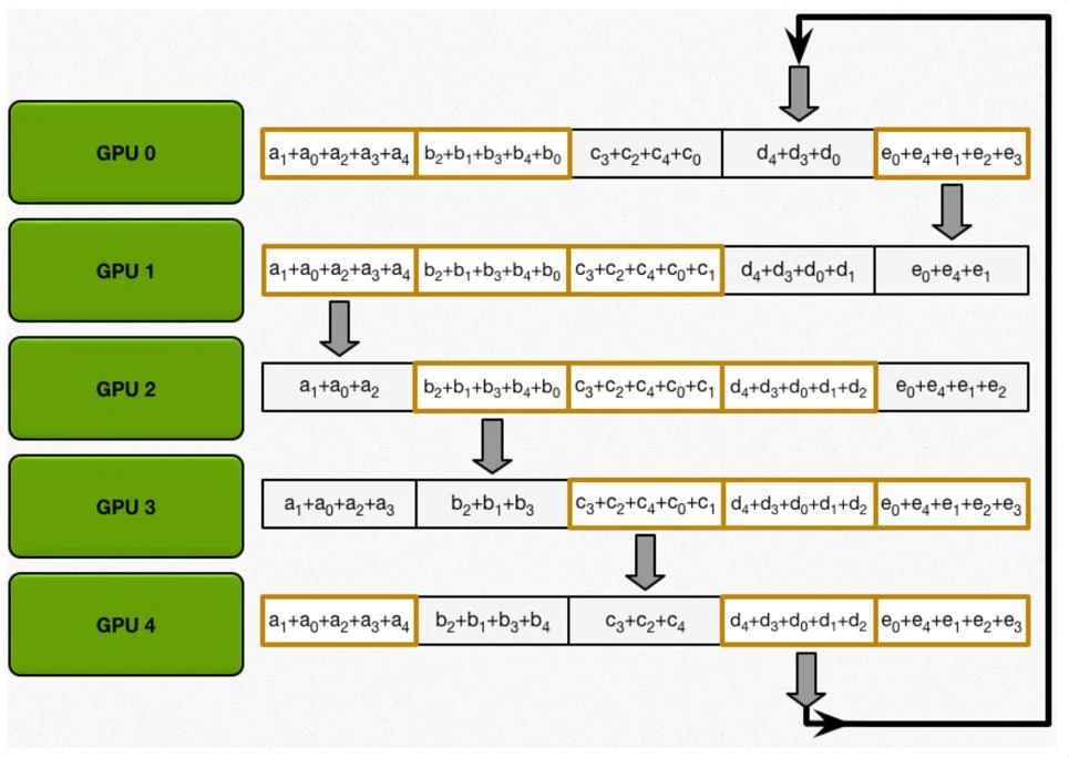
After another
For a gradient containing
values through the server. In a bandwidth-efficient ring, each process transfers approximately
The factor
A physical cluster is not always a one-dimensional ring. A two-dimensional torus creates horizontal and vertical rings so that collective communication can better follow the hardware’s links.
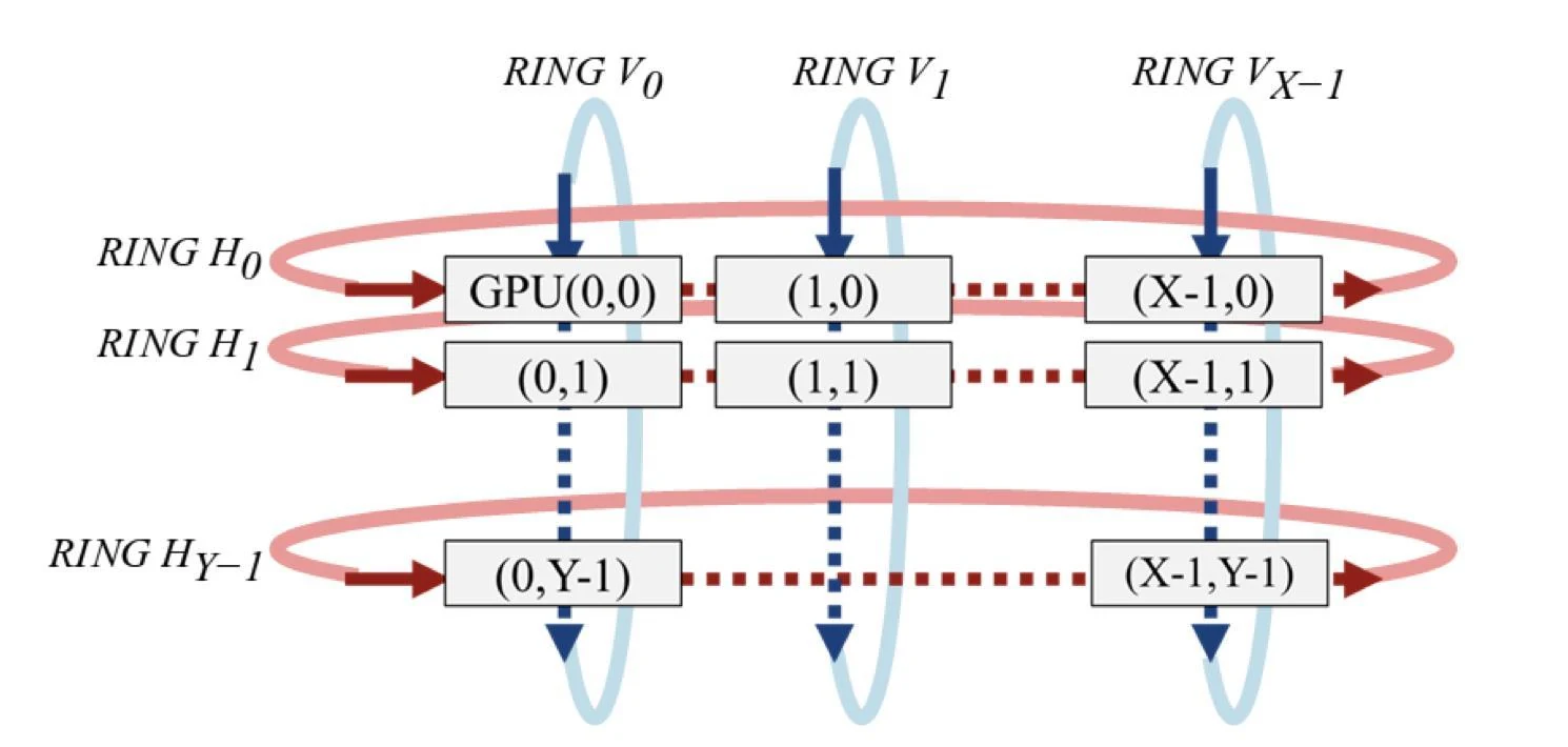
The slide’s
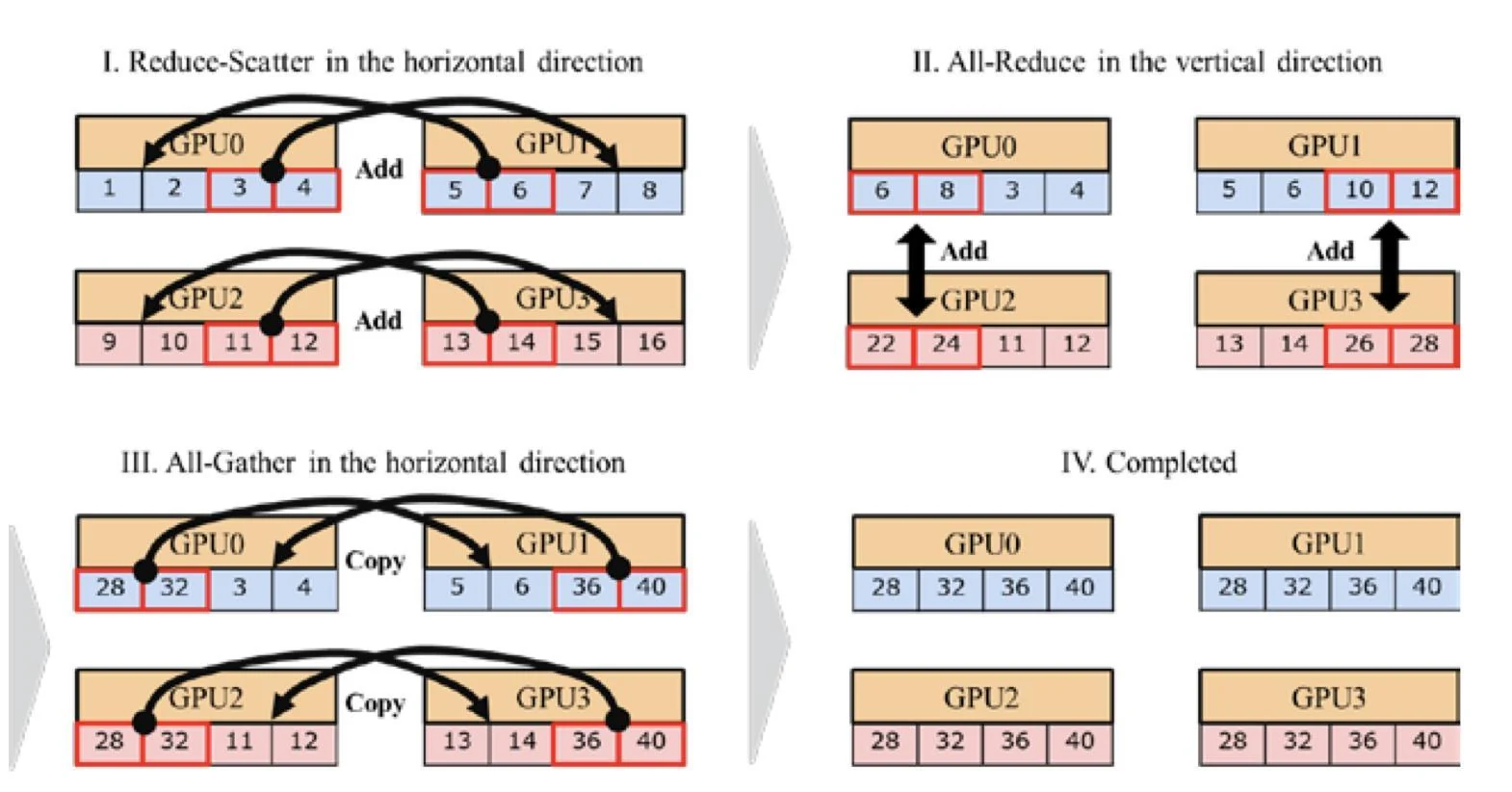
Ring all-reduce is bandwidth efficient for large messages, but its
Benchmark Rules
Benchmarking distributed training requires both statistical and systems controls. Record:
- target accuracy or loss and the size of the test set;
- total training time and time to target quality;
- model, dataset, batch size, precision, and optimizer;
- framework and version;
- accelerator type and count;
- intra-node and inter-node topology;
- communication library;
- throughput, speedup, scaling efficiency, and overhead.
Speedup and scaling efficiency are
Distributed overhead can be estimated by comparing distributed iteration time with corresponding single-device iteration time. Compute-to-communication ratio matters: a larger model or batch can hide communication more easily. Framework compute performance can differ by as much as 50% in the cited comparison. A slower GPU can misleadingly make communication overhead look smaller because there is more compute time to hide it; the slides note that a P100 can be roughly three times faster than a K40 on relevant work.
Strong scaling fixes the total workload and adds workers; weak scaling grows the workload with worker count. They answer different questions and should be labeled. Repeated runs, warm caches, a sufficiently large test set, and disclosed preprocessing prevent noise or hidden work from dominating the conclusion.
ResNet Case Study
The ImageNet/ResNet-50 table illustrates why one number is insufficient:
| Work | Batch | Hardware | Software/network | Time | Top-1 |
|---|---|---|---|---|---|
| He et al. | 256 | 8× P100 | Caffe | 29 h | 75.3% |
| Goyal et al. | 8K | 256× P100 | Caffe2, 50 GbE | 60 min | 76.3% |
| Cho et al. | 8K | 256× P100 | Caffe, InfiniBand | 50 min | 75.01% |
| Smith et al. | 8K→16K | full TPU pod | TensorFlow | 30 min | 76.1% |
| Akiba et al. | 32K | 1024× P100 | Chainer, InfiniBand FDR | 15 min | 74.9% |
| Jia et al. | 64K | 2048× P40 | TensorFlow, 100 GbE | 6.6 min | 75.8% |
| Ying et al. | 32K | 1024× TPU v3 | TensorFlow | 2.2 min | 76.3% |
| Ying et al. | 64K | 1024× TPU v3 | TensorFlow | 1.8 min | 75.2% |
| Mikami et al. | 54K | 3456× V100 | NNL, dual EDR | 2 min | 75.29% |
Some reported scaling efficiencies are about 90%, 95%, 80%, 87.9%, and 84.75%, depending on the experiment. But the table also shows accuracy changes, different batch sizes, frameworks, networks, and accelerators. A faster headline time may use more hardware or end at lower accuracy.
The practical reading is not “the last row wins.” Ask how much hardware was consumed, whether accuracy targets match, whether the global batch changed optimization, how the network was provisioned, and whether the measurement includes input and validation. Only then can the experiments support a fair systems conclusion.
Lecture 1 closes with preparation for Lecture 2: GCP, Colab, course coupons, cloud clusters, and the first homework around September 12. The broader lesson is already established: model quality and system performance must be designed and measured together. A training method is successful only when it reaches the required quality reliably, reproducibly, and at an acceptable resource cost.
- Title: LLM 1 - Fundamentals of Deep Learning
- Author: Gavin0576
- Created at : 2026-09-11 16:15:28
- Updated at : 2026-09-12 14:48:00
- Link: https://jiangpf2022.github.io/blog/2026/09/11/LLM-Based-Generative-AI-Columbia-University/
- License: This work is licensed under CC BY-NC-SA 4.0.