9 - Differential Equations 101

Welcome in. Before we write a derivative, place an imaginary glass of water on the desk and watch its level fall through a small hole. You already understand the story: a high water level creates a strong outflow, the outflow lowers the level, and that lower level weakens the next outflow. A differential equation is the compact language for that feedback.

This blog is not a catalogue of tricks for integrating equations. Its purpose is more practical: to show how a changing system becomes a model. We will move through four examples from the original course material—a pendulum, pursuit at sea, a draining vessel, and a cooling rod—and then use the same grammar for population growth. By the end, you should be able to identify a state, construct its rate law, state the missing initial or boundary information, and decide whether an exact formula or a numerical trajectory is the honest answer.

The modeling sentence

Change = inflow − outflow + generation − loss. Before searching for an equation name, decide what is stored, what crosses the boundary, and what changes the stored quantity internally.

State Equations

A differential-equation model starts with a state: the smallest collection of time-dependent quantities that lets the future be computed once the inputs are known. Position alone is not a complete state for a moving pendulum, because the same angle can be crossed in two directions. Angle and angular velocity are sufficient:

Here denotes an external input and denotes fixed parameters. This notation prevents three mistakes: treating an input as a state, allowing a parameter to change without a rule, and fitting a curve without specifying its mechanism.

Units are the first debugger. If is liters, must be liters per minute. Signs are the second debugger: a loss term must reduce the state.

An th-order scalar equation can be converted into first-order equations. For

set and :

This state-space form is what numerical solvers advance.

Pause before calculating

A cup of coffee cools in a room. Which quantities must be states: coffee temperature, room temperature, cup color, elapsed time? If the room is a huge thermal reservoir, its temperature is an input; in a sealed insulated box, it becomes another state.

The state must remember enough—but no more than enough

The phrase “smallest collection” deserves some patience. Imagine that a campus shuttle is moving along a straight road. If you know only its position at 8:00, you cannot predict its position at 8:01: it may be moving east, moving west, or parked. Position is therefore not a sufficient state. Position and velocity are sufficient if acceleration is prescribed by a known law. If the driver has a delayed reaction, the present position and velocity may still be insufficient because the next acceleration depends on an earlier observation. You could then include the delayed quantity in the state, or use a delay differential equation. The correct state is determined by what the future needs to know, not by the list of columns that happens to be available in a spreadsheet.

This is the Markov property in modeling language: conditional on the current state and future inputs, the future should not need the full past. It does not say that history is irrelevant. It says that the relevant influence of history has been compressed into the state. A battery model may use charge alone at first. If identical charges lead to different voltage responses because of temperature and degradation, charge is not sufficient; temperature and a health variable must be added. A disease model may use current infected population alone. If immunity depends on how long people have been infected, infection age or several staged compartments may be needed.

There is an opposite mistake: declaring every measured quantity a state. Clock time is usually the independent variable, not a state. A fixed vessel radius is a parameter. Rainfall forecast is an input. The color of a tank is irrelevant unless it changes radiation absorption. A bloated state makes calibration harder and hides the mechanism. For each proposed component, ask a sharp question: if I remove this quantity while holding the remaining state and inputs fixed, can two physically plausible futures result? If yes, it carries necessary memory. If no, it may be derived, prescribed, or irrelevant.

The same distinction clarifies notation. In

evolves because the equation tells it how. The input is supplied from outside the model: a pump schedule, ambient temperature, medication dose, or policy intervention. The parameter vector is fixed during one simulation: mass, pipe diameter, growth rate, or heat-transfer coefficient. An observed output

need not equal a state. A sensor may measure only a noisy combination of states. This separation becomes crucial during parameter estimation: the solver advances states, the observation function predicts what the instrument would see, and the residual compares that prediction with data.

Derive the rate from a short time balance

Many students are told to “write the differential equation” as though the equation should appear by recognition. A safer habit is to write a balance over a short interval . Suppose is the mass of dissolved salt in a tank. Over a short interval,

If inflow rate is , inlet concentration is , outflow rate is , and a reaction consumes salt at rate , then

Divide by and take the limit:

Only after this balance should we substitute . If volume changes, gives

so writing alone would silently discard dilution or concentration caused by changing volume. The product rule is not a technical nuisance; it is the mathematical record of what is stored.

The short-interval method also reveals event timing. Suppose a reservoir gate opens at noon. The input is piecewise:

The state normally remains continuous at noon, but its derivative changes. A numerical implementation should integrate to the event, update the input, and continue. Smearing the opening across a large time step changes the physical problem.

Dimensions, signs, limiting cases, and invariants

Before solving, subject the proposed equation to four inexpensive tests. First, every additive term must have the same dimension. In

if is individuals and time is days, then has units day and has units individual day. A fitted value without its unit cannot be transferred between a count measured in individuals and one measured in thousands.

Second, check signs at meaningful boundaries. At , a closed biological population should not become negative. If the equation gives at zero, it violates nonnegativity unless an external removal is explicitly capped. For tank depth , outflow should be zero; a constant negative outflow would drive the model below the empty state.

Third, remove a mechanism and see whether the equation reduces correctly. If drag coefficient tends to zero, a damped oscillator should become an undamped oscillator. If a hole area tends to zero, drain time should diverge. If contact rate tends to zero, infection incidence should vanish. Limiting cases catch algebra that a polished plot can conceal.

Fourth, look for an invariant or balance. For an isolated oscillator,

should remain constant. For a closed compartment system, total mass should remain constant. For a model with known supply and loss, the change in total storage should equal their cumulative difference. These identities are excellent automated tests because they assess the trajectory at every time rather than only the final value.

Consider a rumor on a campus. It is tempting to write because “more informed students tell more people.” But this equation allows informed population to exceed total population. The short-interval story exposes the missing limitation: encounters require both an informed and an uninformed student. A first model might be

At and , the rate is zero; between them it is positive. Units, signs, and limiting cases all agree. Whether homogeneous mixing is plausible remains an empirical question, but the equation now expresses a coherent mechanism.

A rate law is a claim, not a curve-fitting convenience

Every factor in a derivative should answer a sentence: who or what must be present, how often an event occurs, and how much the state changes per event. If a factor has no verbal meaning, the model is not yet ready for computation.

Worked model: bicycles circulating through a campus

Suppose a university wants to prevent an empty bicycle station near the library during the morning rush. At first the problem appears discrete: bicycles are individual objects, riders arrive one at a time, and stations have integer capacities. A continuous differential equation can still be a useful planning baseline when flows are large enough that average rates are meaningful.

Let be the expected number of bicycles at station . Let be the departure rate from station toward station . A balance is

where is truck-based rebalancing into station ; negative means removal. In a closed campus network with no bicycles entering or leaving,

and summing the station equations gives

This invariant is the first code test. If a simulation creates bicycles, a transfer term was not written with opposite signs.

How should demand depend on availability? A naive prescribed departure rate can remove bicycles from an empty station. One smooth approximation is

where controls how sharply departures shut down as inventory approaches zero. Another model uses the requested rate capped by available stock over a short control interval. The smooth form is convenient for analysis; the capped form is easier to explain operationally. Both approximate an underlying queue of customers and integer bicycles, so their validity should be checked against an event simulation.

Capacity creates a second boundary. If station is full, an arriving rider cannot complete the trip there. A physically faithful model needs rerouting, waiting, or lost demand. Multiplying arrivals by an available-space factor such as

prevents overflow in a smooth approximation, but it does not tell us where rejected riders go. A network model should move that flow to alternative stations or record it as unsatisfied demand.

The planning decision is not the prettiest inventory curve. It might be a rebalancing schedule that minimizes truck distance while keeping the probability of an empty or full station below a service target. The ODE can forecast mean inventory under candidate . A stochastic discrete-event model can then test tail risk. This layered approach uses the simple model for insight and the detailed model for service guarantees.

Calibration requires trip start and end timestamps, station capacities, outages, and truck movements. Raw checkout counts do not reveal denied rentals because no transaction is created when a station is empty. If denied demand is ignored, the fitted departure rate falls exactly when unmet demand is highest. External counts, app search logs, or nearby-station diversions can help estimate latent requests.

A useful validation holds out a busy day and reconstructs inventory from the morning count. Compare predicted and observed times of first empty/full event, not only average inventory error. If the model misses those events while matching daily totals, it is not adequate for the decision.

Now connect this example to state sufficiency. If trip durations are negligible, direct station-to-station flows may be acceptable. If trips take twenty minutes, bicycles currently in transit are missing state. Add for bicycles traveling from to , or represent a travel-time delay. Otherwise a bicycle leaves one station and appears at another instantly, shifting peak timing and making rebalancing look easier than it is.

Weather and class schedules are inputs, not states, unless their dynamics are modeled. Station capacity is a parameter. Expected inventory is a state. A customer’s probability of finding a bicycle is an output derived from inventory uncertainty. This classification prevents a common modeling failure: placing every data column into one differential equation without asking what evolves.

Finally test limiting cases. With every demand and rebalancing rate set to zero, inventories must remain constant. With two stations and one constant one-way flow, the origin should empty while the destination fills. If travel time tends to zero, an in-transit model should approach the instantaneous model. If capacity tends to infinity, full-station blocking should vanish. These tests are small, but together they establish much more confidence than one animation of colored bicycle icons.

State-design challenge

A bicycle leaves Station A at 8:00 and reaches Station B at 8:20. At 8:10, should it belong to A, B, or neither station state? If travel time matters to the service decision, the model needs an in-transit state or an explicit delay.

Well-Posedness

The equation specifies possible motion; conditions select the motion that actually occurs. An initial-value problem gives the state at one time,

A boundary-value problem gives information at different locations or times. A steady rod may satisfy and . A second-order equation generally needs two independent conditions. An equation without enough conditions is a road map without a starting point.

Existence and uniqueness matter. If is continuous, a local solution often exists. If it is locally Lipschitz in , nearby initial states do not branch into multiple solutions immediately. The toy equation

has more than one solution because the right side is not Lipschitz at zero: the trajectory may wait and then depart. This is not a solver bug; the model itself does not choose a unique future.

Always state the validity domain. Small-angle pendulum equations fail at large angles. Torricelli outflow assumes a small opening and quasi-steady flow. Logistic growth assumes an aggregated population and a roughly stable environment. These conditions are part of the model.

Why conditions carry physical information

Let us make the counting rule concrete. The equation has the family

Two constants remain because the equation is second order. Giving determines but leaves free; every possible initial velocity still produces a different trajectory. Giving determines . The pair of conditions does not decorate the solution. It tells us which member of the family corresponds to the experiment.

Conditions should be physically independent. Saying twice does not provide two pieces of information. Nor does specifying position and an algebraically equivalent statement about the same position. In mechanics, position and velocity are natural initial conditions. For a beam, position and slope or moment may be specified depending on support type. For diffusion, a boundary can prescribe temperature, heat flux, or a heat-transfer law. The mathematics must match what the apparatus actually controls.

There are three common boundary types. A Dirichlet condition prescribes a value, such as C. A Neumann condition prescribes a flux, such as

A Robin or mixed condition relates flux to the boundary value, for example convection:

Replacing an insulated end, , with a fixed-temperature end changes the whole profile. A report that says only “appropriate boundary conditions were used” hides a central modeling decision.

Conditions also decide whether a parameter can be learned. Suppose Newton cooling is

If and are known, two later temperature measurements can estimate and provide a check. If is unknown and every observation occurs very early, many pairs can trace nearly the same short segment. More data points at the same uninformative time do not fully solve the problem; observations closer to equilibrium help identify .

Existence, uniqueness, and continuous dependence

The formal theorems answer practical questions. Existence asks whether the rules admit a trajectory. Uniqueness asks whether the same initial condition determines only one trajectory. Continuous dependence asks whether small changes in data or initial state produce small changes over the time horizon of interest. Without these properties, “simulate the model” may not be a well-defined instruction.

For the scalar initial-value problem

continuity of near is enough for a local solution under standard conditions. A Lipschitz bound

gives uniqueness. Differentiability with a bounded derivative in is a convenient sufficient condition. The earlier example violates this near zero. Besides , a solution can wait until time and then follow

All these trajectories share when . The ambiguity is not removed by a more accurate Runge–Kutta method. The mechanism needs refinement near zero.

Continuous dependence can be bounded with Grönwall’s inequality. If two solutions satisfy the same Lipschitz dynamics but start at and , then roughly

The exponential is a warning: even a well-posed system can amplify uncertainty over a long horizon. A forecast should not report ten precise digits merely because the numerical solver does. Initial-condition uncertainty, parameter uncertainty, and model discrepancy may dominate discretization error.

Finite-time blow-up is another modeling signal. The equation

has

which diverges at . Sometimes blow-up represents a real threshold outside the model’s domain; often it announces a missing capacity, depletion, or saturation mechanism. Extending the numerical line beyond the singularity is not a forecast.

Algebraic constraints, switching, and feasibility

Not every dynamic model is a pure ODE. Electrical circuits, constrained mechanics, and process networks often combine differential states with algebraic conditions:

This is a differential-algebraic equation. The initial pair must satisfy ; arbitrary starting values can be inconsistent. Eliminating may be possible, but doing so can produce unstable formulas or conceal the constraint. Specialized solvers preserve the coupled structure.

Hybrid models switch equations when events occur. A bouncing ball follows gravity while airborne and a reset rule at impact. A reservoir spills only when level exceeds a crest. A medication schedule changes input at dose times. Write both the continuous dynamics and the event rule:

A time grid that steps over the event can violate mass or place the event at the wrong time. Event detection should locate the zero of a guard function, apply the reset, and restart integration. In a contest model, this detail matters when a threshold determines cost or safety.

Feasibility must also respect physical bounds. If a numerical method produces negative population, clipping it to zero after every step hides instability and destroys conservation. First reduce the step or choose a positivity-preserving method. If a control can remove more stock than exists, cap the removal within the model. If the continuous approximation genuinely permits tiny negative roundoff, report and bound it rather than silently altering the trajectory.

A well-posedness audit before any solver call

Take a simple heated room. Indoor temperature obeys

Before computing, list what is known. The initial indoor temperature supplies one condition for this first-order equation. Weather , heater power , and internal gain are inputs. Heat capacity , conductance , and efficiency are parameters. If a thermostat makes depend on , its switching logic is part of the model. If an open window changes , that event must be recorded or represented as uncertainty.

Now ask what the output will support. One indoor sensor under a single thermostat schedule may identify the ratio more reliably than and separately. A second experiment with a known heating pulse can help. The initial condition must be taken at the true start, not estimated using future data if the intended use is real-time prediction. Each of these choices is part of well-posed modeling even though none requires integrating the equation.

A boundary-condition trap

A metal rod is insulated at its right end, but a model uses the measured right-end temperature as a fixed condition. Both models can fit one snapshot. Which experiment—changing ambient temperature, changing left-end heating, or measuring right-end heat flux—would most clearly distinguish the physical boundary laws, and why?

Worked model: an infusion protocol with a terminal target

Boundary-value thinking appears outside spatial physics. Suppose a drug is infused over six hours and the planner wants concentration to begin at and reach a target , while keeping the infusion rate smooth and nonnegative. A one-compartment model is

If is prescribed, this is an initial-value problem. If must be chosen so that the terminal condition is met, it becomes a control or boundary-value problem. The target does not provide a second condition for the first-order ODE while is known; instead it constrains the unknown function .

For a constant infusion , the solution is

from a zero initial concentration. Enforcing gives

This hand solution supplies a baseline. If there is also an upper concentration limit before , the monotone constant-infusion trajectory satisfies it whenever is within the limit. If rapid arrival at a therapeutic range matters, a loading dose followed by maintenance may perform better, but peak safety and pump limits must be modeled.

Suppose instead that the objective penalizes both terminal error and abrupt control:

The state equation, initial condition, pump bounds, and this objective define an optimal-control problem. A direct transcription can discretize and , but grid refinement and independent reintegration are required. The resulting schedule should be compared with the constant baseline; otherwise complexity has no benchmark.

Now consider parameter uncertainty. If elimination differs among patients, the constant rate calculated at the nominal can underdose fast eliminators and overdose slow eliminators. A robust plan could require a safe concentration band over a credible interval, while an adaptive plan measures concentration and updates . These are different decisions: robustness fixes a plan before uncertainty is resolved; feedback uses later information.

The example also illustrates compatibility. Asking for , , and for every is inconsistent unless . A numerical optimizer may report infeasibility, but the modeler should detect the contradiction before blaming the solver. Likewise, a target above the maximum reachable concentration under is impossible. The reachability bound for constant maximum infusion is

Compute this bound first.

Terminal conditions can be soft or hard. A hard equality may demand a clinically meaningless level of precision and create sensitivity to parameter error. A tolerance band

is often more faithful. A terminal penalty expresses preference rather than feasibility. State why one is used.

Finally, distinguish a measurement at from a true state condition. An assay observes concentration with error and perhaps delay. Forcing the simulated state through a noisy final measurement can distort the trajectory. In calibration, treat the measurement through an observation model; in design, use a clinically defined target. Same number, different epistemic role.

This small protocol shows why “number of conditions equals differential order” is only the beginning. We must ask what is known, what is controlled, what is observed, and what is required. Initial conditions select a trajectory, boundary targets constrain a design, algebraic relations restrict feasibility, and measurements provide uncertain evidence.

The Pendulum

Take a point mass on a massless rod of length . Let be measured from the downward vertical. Tangential gravity is , so

For small , use :

With and ,

and

Mass disappears, but length remains. The approximation also erases amplitude dependence. For initial amplitude ,

If required timing precision is tighter than , the linear approximation is inadequate.

The state is not merely angle: angle and angular velocity determine the next motion.

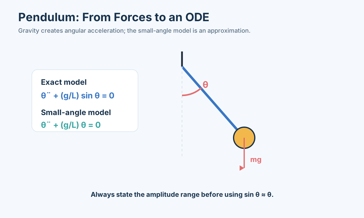
Build the equation from torque, not memory

Let us repeat the derivation slowly enough that every sign can be defended. The bob position relative to the pivot is

Gravity is . The scalar torque about the pivot is the out-of-plane cross product

The moment of inertia of a point mass at distance is . Rotational Newton’s law gives

After cancellation, . The negative sign is now inevitable: for a small positive angle, gravity creates a negative angular acceleration toward the bottom. If your coordinate convention measures from the upward vertical, both the potential and stability change. A diagram should be drawn before a sign is chosen.

Energy provides an independent derivation and a verifier. Kinetic and potential energy are

Differentiate :

Thus the exact ideal trajectory stays on a constant-energy contour. A numerical solution whose energy steadily grows is injecting artificial energy; one whose energy steadily shrinks has numerical damping. This does not automatically make a method useless, but the error must be smaller than the effect being studied.

At the turning point and . Conservation gives

This relation reduces the period calculation to an integral. It also supplies a pointwise check: at the bottom, speed should satisfy

If a simulation at amplitude produces a larger bottom speed without external forcing, either the units, initial condition, or integrator is wrong.

What the small-angle approximation spends

The Taylor expansion

shows the first discarded term. The approximation error is not “small” in the abstract; it is small relative to a required decision tolerance. At radians, the relative force error is about . At radians, it is about . Degrees must never be substituted directly into a Taylor formula written in radians.

The linear equation has angular frequency . Its period follows from one complete cosine cycle:

Dimensional analysis almost predicts the square root. The only available quantities are length and acceleration with units and . The combination with time units is . Dimensional analysis cannot produce , but it rules out immediately.

The exact period can be written using the complete elliptic integral. Expanding it gives

Suppose a timing experiment needs error below . Keeping only the first correction suggests , or radians, about . This turns an approximation statement into an experimental design rule.

Damping, forcing, and resonance

Real pendulums lose energy. A common model adds viscous torque :

For small angle, divide by and define

When , the unforced response oscillates with decaying envelope and damped frequency . At , critical damping returns toward equilibrium without oscillation as quickly as possible in the linear model. Larger is overdamped and slower. These regimes can be identified from data more reliably if several cycles or the full relaxation are observed.

With sinusoidal forcing , the steady-state amplitude is

Resonance is not simply “forcing frequency equals natural frequency” once damping is present. The displacement-amplitude peak occurs near when damping is light enough. Near resonance, parameter and frequency uncertainty matter greatly; a tiny detuning can change amplitude. A safe design reports an amplitude curve over a frequency band, not one nominal point.

A complete experiment and model comparison

Imagine recording phone video of a pendulum released from , , and . Extract angle versus time and timestamp uncertainty. Before fitting, predict: the linear model should give one amplitude-independent period; the nonlinear model should give increasing period; damping should shrink peaks. These qualitative predictions prevent blind optimization.

Fit three nested models: linear undamped, linear damped, and nonlinear damped. Use the first experiment for calibration and the others for validation. Compare phase error after several cycles, peak decay, and energy balance. A model may match the first two peaks yet accumulate timing error. Report residuals against time and angle; residual dependence on amplitude is evidence that the small-angle approximation is inadequate.

Parameter identifiability matters. The undamped period estimates , not and independently. If is measured, can be inferred; if neither is known, infinitely many pairs share the same ratio. Damping-envelope data estimate , so estimating separately requires mass and length. Optimizer precision does not overcome this algebraic limitation.

Finally compare with a deliberately simple baseline: estimate the period by time between every other zero crossing. If a sophisticated nonlinear fit does not improve held-out phase prediction beyond timestamp error, the extra machinery has not earned its place. If it does, show where—in amplitude dependence, damping, or forced response—the improvement matters.

Pendulum evidence chain

The torque diagram justifies the ODE; energy checks the implementation; the small-angle remainder defines the approximation range; repeated amplitudes challenge that range; and held-out cycles test whether fitted damping predicts rather than merely reconstructs.

Worked calculation: when does linearization change the decision?

Imagine designing a pendulum-based timing gate that must predict the tenth return to the release side within 0.10 seconds. The pendulum length is m and release amplitude is . The small-angle period is approximately

Convert amplitude to radians: . Using the first two corrections,

The period increase is about s. After ten cycles, the small-angle prediction is early by roughly s, far beyond the tolerance. For a classroom demonstration of one swing, the approximation might be fine; for the timing gate, it is not. Approximation quality belongs to the decision horizon.

Suppose damping reduces amplitude over those ten cycles. Then the nonlinear period gradually approaches . Simply multiplying the first-amplitude correction by ten overestimates phase error. We need the damped nonlinear ODE. This is a useful escalation rule: start with the hand bound; only simulate the more detailed mechanism when the bound threatens the decision.

Use the state

with

Detect returns using an event with positive-to-negative crossing and . Event direction prevents counting the opposite turning point. Record event times and compare linear, nonlinear undamped, and nonlinear damped models.

Before using experimental data, test the undamped simulation. Energy relative error

should shrink as solver tolerance tightens. Event times should converge. If the method preserves angle visually but drifts in energy, the tenth-return metric may still be wrong.

For video calibration, model timestamp and angle extraction. If frames arrive every s, individual turning times cannot be known to arbitrary precision. Sub-frame interpolation helps, but the uncertainty should appear in parameter intervals. Lens perspective and pivot location cause systematic angle error; calibrate geometry using known points or restrict motion to a plane perpendicular to the camera.

Fit length only if it was not measured accurately; otherwise use the physical measurement and fit damping. If both and are free, period identifies their ratio. If a fitted “gravity” differs greatly from m/s, this may signal an effective length, pivot inertia, or camera timing error rather than local gravity.

Compare phase residuals, not only angle residuals. A small frequency bias creates alternating angle errors and large long-horizon phase drift. Plot predicted versus observed turning times across cycles. If early cycles match but later cycles drift, frequency or amplitude dependence is wrong. If amplitudes decay at the wrong rate, damping law is wrong. If both vary with direction, pivot friction may be asymmetric.

Dry friction behaves differently from viscous damping. A Coulomb torque has nearly constant magnitude opposing motion:

It can produce approximately linear amplitude decay and sticking near equilibrium, while viscous damping produces exponential decay. A model with both terms may be needed, but compare their signatures before fitting extra coefficients.

Report the final conclusion in decision language: the small-angle model misses the tenth return by more than the allowed tolerance at ; the nonlinear damped model predicts held-out return times within measurement uncertainty for releases between specified amplitudes; outside that range no guarantee is claimed. This is stronger than saying one model has a lower mean squared error.

Pursuit Curves

Suppose a submarine travels at constant speed along course , while a patrol boat of speed always points directly at it. Let

be the target and the patrol boat. “Always points directly” becomes

Define relative displacement :

For distance ,

Since , guarantees closing. In the course example, 60 knots versus 30 knots guarantees eventual interception, but the path and time still require integration.

A line-of-sight pursuit creates a curved tail-chase. A lead-intercept strategy aims at a predicted meeting point and can be shorter, but requires knowledge of target course. A competition model should compare the strategies and state what information each needs.

The normalized line-of-sight vector turns the pursuit story into an ODE.

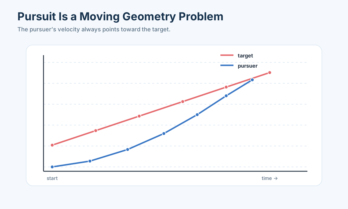
Turn a verbal navigation rule into a vector field

The patrol boat example contains two different questions that are often mixed. The first is a policy: where should the pursuer point at each instant? The second is an outcome: under that policy, when and where will interception occur? “Always point at the current target” answers the first. The ODE calculates the second.

Write both positions in the same coordinate frame and use the same time unit. If one knot is one nautical mile per hour, speeds of 60 and 30 knots should not be combined with seconds unless converted. Let the target start at and move on heading unit vector . Then

For pure pursuit, the pursuer velocity has fixed magnitude and line-of-sight direction:

The normalization is essential. Using would make speed proportional to distance and give the wrong units. At interception the denominator vanishes, so the integration should terminate when reaches a declared capture radius rather than stepping through the singularity.

Relative coordinates simplify reasoning. With ,

Let and let be the angle from the target heading to the line of sight, so . Then

Because , the conservative bound

guarantees capture when . Integrating this inequality gives

For the 60-nautical-mile separation and speeds 60 and 30 knots, pure pursuit must intercept within two hours. This bound is not necessarily the actual capture time, but it is a powerful simulation check. A computed time longer than two hours contradicts the inequality.

Pure pursuit versus lead interception

If the target course and speed are known, the pursuer can aim at a predicted meeting point. For constant pursuer heading unit vector , interception requires

Let . Taking norms after rearrangement gives

Expanding produces a quadratic:

Choose the smallest positive root and set

This lead policy is direct when the prediction is correct. Pure pursuit uses less information and continually corrects, but wastes motion following the target’s wake. A proportional-navigation law uses line-of-sight rotation and is common in guidance problems. The “best” policy depends on observation noise, maneuverability, fuel, capture radius, and uncertainty in target behavior.

A revealing experiment perturbs the target heading after half an hour. The original lead heading can miss badly unless replanned; pure pursuit adapts immediately; a receding-horizon lead policy recomputes the intercept using new observations. Compare capture time and path length over a set of maneuvers instead of declaring a winner from one straight trajectory.

Numerical implementation and evidence

Integrate the four state components or the two relative components. An adaptive solver should stop at event

At each output time verify pursuer speed:

Also verify target straightness, monotone distance under , and the analytical upper bound. Run step-tolerance refinement because capture time is an event estimate. Plot trajectories with equal axis scales; otherwise a shallow curve may appear dramatic or a large detour may look small.

If observations arrive intermittently, distinguish true state from estimated state. A tracker supplies and perhaps ; guidance uses those estimates. Measurement noise can make the direction chatter when distance is small. Filtering, a capture radius, and acceleration limits turn a geometric demonstration into a physically plausible system.

Navigation decision

The target is faster than the pursuer but must reach a known harbor while the pursuer can choose an intercept point. Pure pursuit may fail because . Can interception still be possible? Sketch the target arrival-time circle and the pursuer reachable circle; the answer depends on geometry and destination, not speed comparison alone.

Worked mission: interception with uncertain heading and turn limits

The ideal patrol boat can rotate its velocity vector instantly. A real vessel has a maximum turn rate. Let heading be and control be yaw rate:

Pure pursuit now becomes a desired heading

followed through a bounded controller such as

Angle wrapping matters: the error between and is , not . A missing wrap can command a full turn in the wrong direction.

Suppose the target heading estimate is with uncertainty and speed uncertainty knots. A single nominal lead point is not sufficient. Simulate coherent scenarios: left and right heading bounds, slow and fast target, and plausible coupled maneuvers. Independent random heading at every second would create physically impossible jitter unless target turn dynamics permit it.

Define mission outcomes before simulation. Capture occurs when . Fuel proxy can be path length plus turn effort,

Safety may require staying outside a restricted region. Failure includes no capture before horizon, fuel limit, or boundary violation. Compare pure pursuit, fixed lead, and receding-horizon lead under exactly the same scenarios.

A receding-horizon policy estimates target velocity from recent observations, calculates a feasible intercept accounting for turn rate, executes for a short interval, and replans. It often combines lead efficiency with feedback. But noisy velocity estimates can send the intercept point from side to side. Filtering and a penalty on heading change may improve behavior.

Use paired scenario differences. For scenario , let and be pure-pursuit and lead capture times. Plot . This reveals whether lead consistently helps or wins only under nominal straight motion. Report failure probability or count only if a defensible scenario distribution exists; otherwise report performance over named cases and worst credible outcomes.

Check the simulation with geometric bounds. The pursuer path length must be if speed is fixed. Target displacement must match its integrated velocity. Without turn constraints and under a straight known target, receding-horizon lead should approach the analytic intercept. As tends to infinity, bounded-heading pure pursuit should approach the ideal ODE.

Observation delay can be modeled by guidance using . Delay increases miss distance and can destabilize aggressive steering. Sweep over measured or credible values. If success collapses above a small delay, the recommendation should include sensor-update requirements, not merely a trajectory.

This extension illustrates a general rule: a kinematic equation can answer “where would an ideal point move?” A deployable policy also needs actuation, sensing, delay, constraints, and failure definitions. Add those layers only as the decision demands, and verify that each new layer changes an interpretable quantity.

Hemisphere Drainage

A hemispherical tank of radius drains through a bottom hole of area . Let be water depth. The horizontal cross-section satisfies

so

The volume rate is . Torricelli’s law gives

Conservation yields

The same volume loss produces different depth loss because cross-section changes. Separating variables and integrating from to zero,

Thus : doubling hole area halves drain time, while doubling radius multiplies it by . Data can estimate ; structured residuals reveal where the outflow approximation fails.

The state equation combines hydraulic outflow with changing vessel geometry.

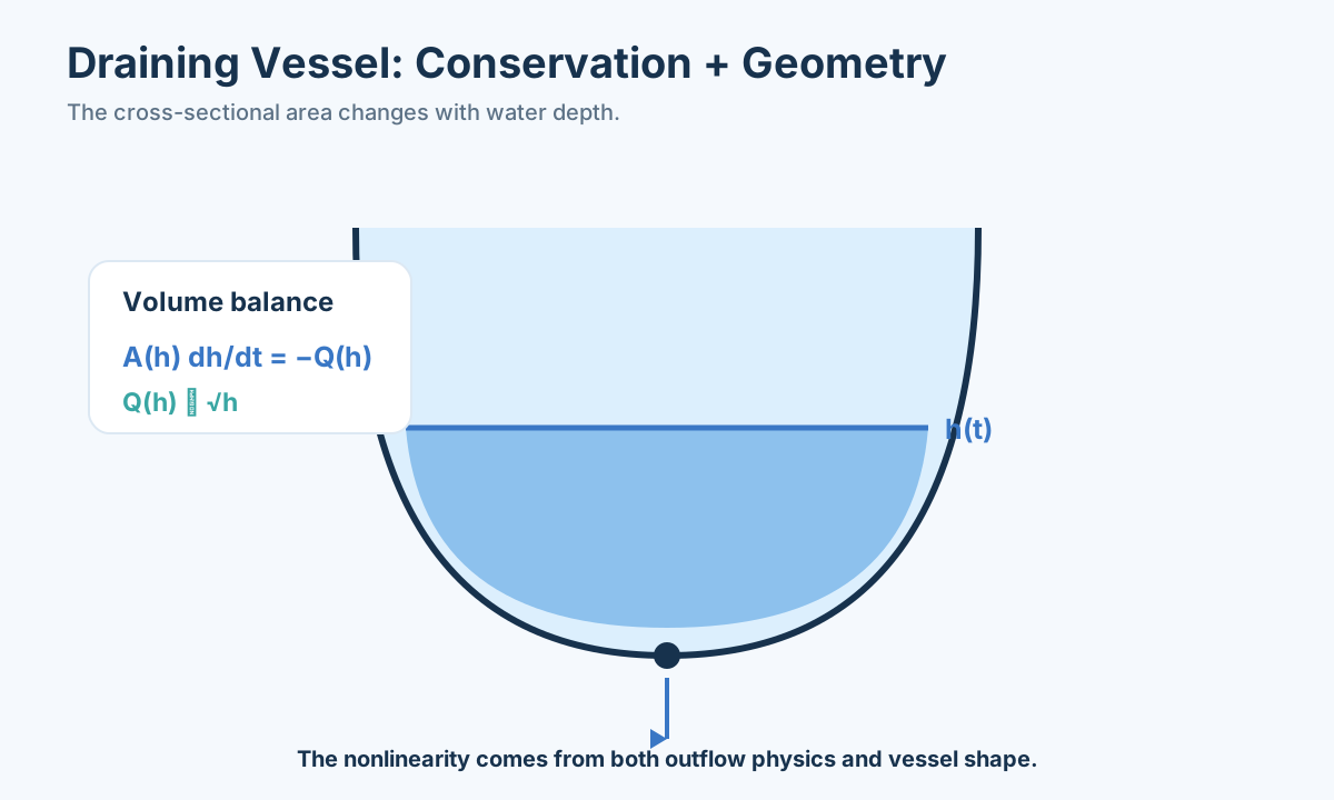
Geometry is part of the dynamics

The draining problem is an excellent antidote to formula hunting. If we guessed from Torricelli’s law, we would be treating every vessel as a vertical cylinder. Torricelli determines volume flow, while the vessel geometry converts volume flow into depth change.

At depth , the sphere center is above the bottom. The circular slice radius follows from the right triangle

so . The cross-sectional area is . The stored volume can also be integrated:

Differentiating recovers . This provides two independent routes to the same geometric factor.

Torricelli’s ideal exit speed comes from converting hydrostatic head into kinetic energy. A discharge coefficient accounts for contraction and loss, giving

Mass conservation for incompressible water is . By the chain rule,

Near the bottom, while outflow is proportional to , so

The ideal depth derivative becomes unbounded as , even though volume flow goes to zero. This is a geometric effect: the cross-section shrinks faster. It also warns that the quasi-steady model and point-hole geometry are least trustworthy at the final instant. A numerical solver should stop at a small depth tolerance and use the analytical remaining-time estimate.

Integrate carefully and check the scaling

Rearrange the equation:

To drain from to ,

The antiderivative is

For a full hemisphere, and , producing

Check units: has units . The result scales inversely with hole area and with the square root of gravity. If a derived expression contains density for an incompressible gravity drain with the same fluid on both sides, ask why; density cancels in the energy balance.

Dimensionless variables make the universal shape visible. Let and define

Then

All hemispherical tanks follow this same nondimensional curve. Radius and hole area only rescale time. If experiments at different sizes do not collapse after scaling, may depend on Reynolds number, the hole may not be geometrically similar, or another mechanism matters.

From textbook tank to measurement model

Suppose depth is recorded every five seconds by an ultrasonic sensor. Do not fit the derivative computed from noisy depth differences; differentiation amplifies noise. Instead integrate the ODE for candidate and compare predicted depths at observation times. Include a possible sensor offset :

Calibrate on one run and validate at another initial depth. If the same coefficient fails systematically near the top, inflow conditions or surface motion may matter. If it fails near the bottom, finite-hole geometry and sensor dead zone are suspects. Plot residuals against depth, not only time, because the mechanism depends on depth.

Several extensions follow from the same balance. With inflow ,

An equilibrium exists when inflow equals outflow. With two holes at different elevations, each activates only when water lies above it, creating a piecewise ODE. With a pump whose curve depends on head, replace the square-root law by measured pump performance. The conservation skeleton stays; only the constitutive flow law changes.

Three layers of the tank model

Conservation says how storage changes. Geometry says how volume relates to depth. Hydraulics says how head produces flow. Keeping the layers separate makes it clear which assumption to revise when data disagree.

Worked design: choose an outlet without creating a new problem

Suppose the hemispherical tank stores process water. Operations require it to drain from full to 10% depth in no more than 18 minutes, but peak outlet flow must stay below downstream capacity . The design variable is hole area .

For depth , flow is

It is largest at the initial full depth , so the downstream constraint is

or

The time to drain from to is

This has form , so the time requirement gives a lower bound . A feasible passive outlet exists only if . Compute that compatibility before optimizing cost.

If the interval is empty, making the hole larger solves time but violates downstream capacity; making it smaller protects downstream but drains too slowly. The model has exposed a design conflict. Possible changes include a throttling valve, temporary downstream storage, a two-stage outlet, or relaxed operational timing. An optimizer cannot make contradictory physics disappear.

A simple passive orifice has high initial flow and low late flow. A controlled valve can target nearly constant downstream flow:

up to hardware limits. The required opening grows as the head falls. Near empty, the formula demands an unbounded area, so the valve saturates and the tail slows. A piecewise control law is more realistic:

Integrate each regime and match at the switching depth. The controlled design may satisfy both peak and time constraints with a smaller downstream burden.

Uncertain changes flow and drain time in opposite operational senses: lower reduces peak flow but increases time. To guarantee both constraints over , use for the peak-flow check and for the drain-time check. Using the same “worst” endpoint for every constraint is incorrect.

Manufacturing tolerance in hole diameter matters quadratically because . A 2% diameter error creates about a 4% area error. Propagate tolerance explicitly and inspect whether the feasible interval still contains a manufacturable design.

The discharge coefficient may depend on geometry and Reynolds number, so validate with a drawdown test. Estimate from the full depth trajectory rather than one noisy instantaneous flow. Plot the transformed relation suggested by the integrated model and residuals against head. If coefficient changes systematically at low head, use a head-dependent curve or restrict the validated operating range.

Report the final design as nominal diameter, manufacturing tolerance, assumed range, predicted drain-time interval, peak-flow interval, and test protocol. This is more useful than one calculated area. It also shows how a differential equation becomes a feasibility argument before it becomes an optimization problem.

Cooling Rods

Consider a rod of length , cross-sectional area , exposed perimeter , conductivity , ambient temperature , and endpoints , . Fourier conduction is

For a differential slice, conduction in minus conduction out minus convective loss is zero:

Therefore

Let and :

Applying both endpoint conditions gives

This is a spatial ODE because steady state removed time. If warm-up matters, conservation produces a PDE with . “Temperature after equilibrium” and “temperature during heating” are different questions.

A differential slice converts conduction and surface loss into the governing equation.

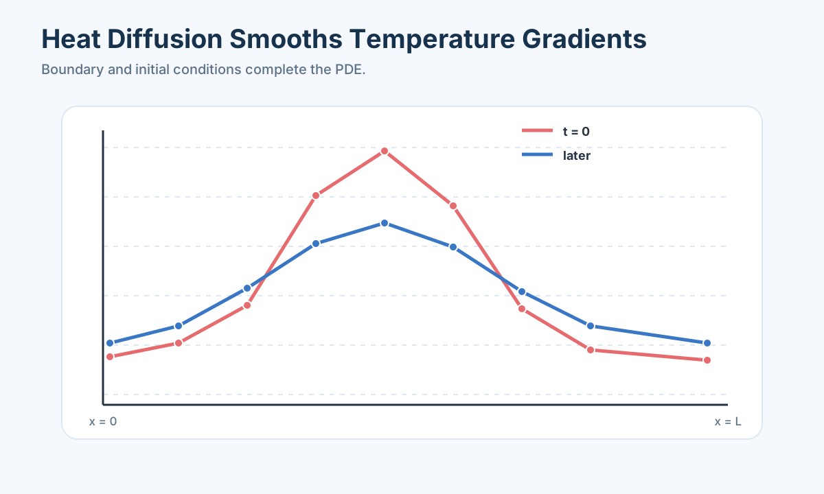
Derive the fin equation from one slice

Take a slice from to . Let positive conductive heat flow point in the positive direction. Fourier’s law gives

At steady state, heat entering at minus heat leaving at minus heat lost from the lateral surface is zero:

Expand , divide by , and take the limit:

Substitute Fourier’s law. If and are constant,

If conductivity or cross-section varies, do not pull it outside the derivative:

That conservative form is the one to discretize. Expanding it incorrectly can violate interface heat-flux continuity.

Set and . The characteristic equation gives

The hyperbolic form is convenient for two endpoint temperatures. The solution already shown can be checked immediately: at the first ratio is one and the second zero; at they swap. Substitution gives . These boundary and equation checks are faster than trusting a symbolic simplifier.

Interpret the dimensionless group

Let . Then

The group

compares lateral convection with axial conduction. When , conduction keeps the rod close to a linear interpolation between endpoints. When , lateral loss pulls much of the rod toward ambient and endpoint influence is localized. This interpretation is more transferable than memorizing the closed form.

Units confirm the group is dimensionless. Heat-transfer coefficient has units W m K, perimeter has m, conductivity has W m K, and area has m. Thus has m.

Consider an insulated tip rather than a fixed right temperature. The boundary condition is . If the base at is , the excess-temperature profile becomes

Heat removed at the base is

For very long fins, : adding length eventually yields little extra heat transfer. This is a genuine design conclusion obtained from the asymptote.

Steady ODE or transient PDE?

The steady equation assumes every slice stores no net energy. During warm-up, storage cannot be ignored. With density and specific heat ,

The initial temperature profile is now required in addition to spatial boundary conditions. A modeler should choose the steady ODE only if the decision concerns equilibrium or if the thermal relaxation time is short relative to operation.

The diffusion time scale is roughly

If measurements are taken after many , steady state may be reasonable. If a reflow oven carries a board through zones on a comparable time scale, transient dynamics are the entire problem.

Discretization as a balance, not a formula

For a uniform grid , a centered approximation gives

But the finite-volume view is safer: compute heat flux at each cell face and balance it with side loss. It handles changing and naturally and preserves conservation across material interfaces. Refine the grid until the temperature profile and base heat rate change negligibly relative to the decision tolerance.

Validate with special cases. Setting should recover a straight line for fixed endpoint temperatures. Equal endpoint and ambient temperatures should yield a constant. Reversing hot and cold endpoints should reverse the profile appropriately. Integrated lateral heat loss plus right-boundary heat flow should equal heat entering from the left. A beautiful temperature curve that fails this balance is not evidence.

Choose the right model

A thin metal fin reaches an apparently stable profile in two minutes, but the design cycles every twenty seconds. Should the steady solution be used to estimate peak temperature? Compare the operation time with the measured or estimated thermal time scale before deciding.

Worked design: sensor placement and insulation diagnosis

Suppose engineers know endpoint temperatures and geometry but do not know the effective lateral heat-transfer coefficient . They can install only two interior sensors. Where should those sensors go, and how should be estimated?

The steady solution depends on . If is very small, the profile is almost linear and weakly sensitive to . Sensors clustered near one endpoint provide nearly redundant information. If is large, most curvature occurs near the hot boundary while the middle approaches ambient. Placement should be guided by sensitivity

Choose points where sensitivity magnitude is appreciable and the two sensitivity patterns are not redundant with uncertainty in endpoint temperatures. A practical design can evaluate candidate locations over a credible range of and maximize a determinant or minimum information criterion.

After measurements , estimate by minimizing

But first include calibration offsets if sensor bias is comparable to the temperature differences. Repeating measurements reduces random noise, not a shared bias. A reference bath or sensor swap helps distinguish position effects from instrument effects.

Now suppose the fitted profile is consistently warmer than predicted near the middle but matches endpoints. Several explanations compete: lower lateral convection, higher conductivity, contact resistance at endpoints, internal heat generation, or an incorrect ambient temperature. Because contains the ratio , a single steady profile may identify that ratio more strongly than either parameter separately. Independent conductivity data or a transient experiment can separate them.

A damaged insulation patch creates spatially varying . Fitting one constant may average the effect and leave localized residual structure. Divide the rod into a small number of zones only if resolution supports it. At each interface, enforce temperature continuity and heat-flux continuity:

Failure to enforce flux continuity creates or destroys heat at the interface.

For design, perhaps the objective is to keep every point above a minimum process temperature while minimizing insulation material. Thickness affects both lateral loss and geometry. A baseline evaluates a few uniform thicknesses. A variable-thickness design can be discretized, but manufacturing smoothness and minimum thickness must be constrained. Validate the final profile with a conservative heat-loss coefficient and a refined mesh.

Do not optimize against the same sensor data used to choose the model without an independent check. Hold out one operating condition, such as a different endpoint temperature or ambient airflow. A physically meaningful coefficient should predict the new profile within uncertainty. If it changes with every condition, the constant-coefficient model is absorbing omitted physics.

The reporting figure should show measured points with error bars, calibrated profile, held-out prediction, and the safety threshold. A separate residual plot should retain spatial order. A table should list units, parameter intervals, and boundary conditions. These elements let a reader reconstruct the evidence rather than admire one smooth curve.

The lesson extends to inverse problems generally. Parameter information comes from how outputs change, not from the number of decimal places in the optimizer. Experimental inputs and sensor locations should excite and observe distinct mechanisms. When two parameters appear only as a ratio, new experimental conditions—not more iterations—are needed.

Population Growth

The simplest population hypothesis is constant per-capita net growth:

This Malthus model can work over short periods with abundant resources. Plotting against should be roughly linear.

For resource limitation, let carrying capacity be :

Separation gives

Growth is fastest at because

A sigmoid curve alone does not prove logistic biology. Product adoption and cumulative cases can also be sigmoid for different mechanisms.

Model comparison

Five increasing measurements are all far below an unknown carrying capacity. Can they distinguish exponential from logistic growth? Usually not. What later observations or external capacity information would make identifiable?

Begin with the event behind per-capita growth

Suppose is a population count. Over a short interval, births contribute approximately and deaths contribute . Then

so with . The important assumption is not merely that the curve is exponential. It is that every individual experiences roughly the same constant net rate, independently of population size and time. The solution follows by separation:

The doubling time is for . If a bacterial culture doubles every 40 minutes, min. If a city grows 2% per year in discrete annual reports, using is an approximation; the exactly equivalent continuous rate is . State which convention is used.

Exponential growth is often a local model. A culture with abundant nutrients, an invasive species immediately after introduction, or cumulative capital under fixed continuous interest may follow it temporarily. Long-horizon extrapolation is dangerous because its mechanism assumes no changing resource, crowding, policy, or behavior. The correct criticism is not “exponential growth is unrealistic.” It is “the constant per-capita-rate assumption is unsupported beyond this regime.”

To model crowding, suppose per-capita growth decreases linearly with population:

Multiplying by gives the logistic equation. Here is the population at which births and deaths balance under the aggregated assumptions. It is not automatically a fixed ecological constant; food, habitat, technology, or policy can make time-dependent.

Separate variables:

Partial fractions give

where the second term is integrated with its sign accounted for. The result is

Using yields

and solving for gives the stated logistic formula. Deriving it once prevents common errors such as reversing the exponential sign or replacing with its reciprocal.

Read the phase line before reading the formula

For and , equilibria are and . The sign of

tells the story. For , , so population increases. For , , so it decreases toward . At zero, no individuals appear spontaneously. A one-dimensional phase line communicates this long-run behavior without solving the equation.

The absolute growth rate is a concave quadratic in . Differentiate:

The maximum occurs at with value . This is the inflection point of the cumulative sigmoid. Before , growth accelerates; afterward it remains positive but decelerates. A plotted curve can look “almost saturated” long before it is close to , so uncertainty bands and residuals matter.

Suppose a renewable population is harvested at constant rate :

Equilibria solve . There are two positive equilibria when , one repeated equilibrium at , and none above it. The number is the maximum sustainable yield in this ideal model. Operating exactly there is fragile: parameter error, environmental shocks, or measurement delay can move the system into decline. A prudent policy stays away from the theoretical boundary and uses feedback.

Proportional harvest produces

If , the positive equilibrium is . If , extinction becomes the only nonnegative equilibrium. Constant and proportional harvesting answer different operational rules; selecting one because it is algebraically convenient can reverse the management conclusion.

Estimating growth parameters without fooling yourself

For exponential growth with multiplicative measurement noise, regressing on time can be appropriate. With additive noise on the original count, log transformation changes the error model and overweights small counts. State what the instrument measures and choose likelihood accordingly.

For logistic growth, a traditional linearization uses

but is usually unknown and measurement error becomes distorted. Nonlinear least squares or likelihood on the original observation model is generally clearer:

Bounds , , and encode physical plausibility, but they do not create information. If every observation satisfies , then

and the data reveal while leaving nearly free. A profile-likelihood plot for will be flat toward large values. Reporting one sharply rounded from such data is misleading.

Design observations around the inflection region if estimating matters. External evidence about habitat or resource capacity can also constrain it. Use held-out late observations to challenge an exponential fit: both models may match early growth, but their forecasts separate near saturation. Compare predictive error, not only in-sample .

Residual pattern helps diagnose missing mechanisms. Seasonal waves suggest time-varying . Repeated crashes may indicate harvesting, disease, or environmental events. Several sigmoids superposed can arise from subpopulations with different start times. An apparent decline in may be observation saturation rather than biological capacity. Each alternative proposes a different data collection plan.

Beyond the basic logistic curve

An Allee effect represents difficulty at low population, for example mate limitation:

Now is an unstable threshold. Below it, population declines; above it, population tends toward . Conservation strategies based on ordinary logistic recovery can fail if the population is pushed below .

Delayed density dependence can oscillate:

The state must include a history segment of length , not only present . A large delay allows the population to keep growing after capacity pressure has become inevitable and keep declining after conditions improve. This is precisely the state-memory issue from Section 1.

Time-varying capacity can model seasonality or habitat change:

When changes rapidly, population lags; it does not simply equal the moving capacity. Scenarios for should reflect coherent environmental futures rather than independent noise at each time step.

Stochastic birth and death matter when counts are small. A deterministic ODE predicts fractions and smooth trajectories; a continuous-time Markov chain models random event times and extinction probability. Deterministic and stochastic models can share the same mean-field rate law but answer different questions. If the decision concerns probability of extinction, the deterministic equilibrium alone is insufficient.

What a sigmoid does—and does not—prove

A sigmoid is a geometric pattern, not a mechanism. Logistic crowding, innovation diffusion, epidemic depletion, a mixture of adoption cohorts, and sensor saturation can all create S-shaped curves. Defend the state and rate law with independent evidence before interpreting fitted parameters.

A small worked comparison

Suppose counts at days are . Early ratios are close enough that an exponential baseline is plausible. From endpoints,

This predicts day 10 count . A logistic model with the same initial slope but predicts a lower value as crowding appears. With only the first four points, , , and a very large may all fit reasonably. The decisive evidence is not another optimizer; it is later measurement near the point where predictions diverge.

Now imagine day 10 count is 52. This challenges pure exponential growth but does not prove . Maybe capacity is near 60, maybe weather temporarily reduced , or maybe the sensor undercounted high density. A good report fits alternatives, checks metadata, and describes which future observation would discriminate among them. Modeling ends with a testable claim, not a curve label.

Worked management case: a fishery with uncertain recruitment

Consider a lake fishery that wants to set next year’s harvest quota. The decision must balance catch with risk of pushing spawning biomass below a recovery threshold. Let be exploitable biomass in tonnes. A first continuous model is

If the quota is implemented as a constant catch , the phase-line analysis above applies. The sustainable equilibrium equation is

Solving the quadratic gives

For , two equilibria exist. The larger is stable and the smaller unstable. If a disturbance drives biomass below , net growth cannot keep up with constant removal and collapse follows. Therefore “below maximum sustainable yield” does not mean safe from every initial state.

Draw the growth parabola and a horizontal harvest line. The vertical distance is . At tangency , the two equilibria merge and recovery is extremely slow near . Parameter uncertainty can turn nominal tangency into no equilibrium. This picture explains why operating at theoretical maximum yield is fragile.

A proportional effort model is often more realistic:

where is fishing effort and catchability. Then

The positive equilibrium is

when . Equilibrium catch is

again a concave curve. Maximum occurs at and . Effort control reduces harvest automatically when stock is low, unlike a fixed catch, although economic pressure may increase effort when catches fall.

The continuous logistic model aggregates age structure and seasonal recruitment. Fish reproduce in pulses, juveniles and adults have different survival, and catch selects sizes. A discrete annual baseline may be

but this Euler-like update can behave unrealistically for large . A Beverton–Holt or Ricker recruitment relationship may better represent annual cohorts. Model choice should follow biology and sampling interval.

Suppose only annual catch and a noisy abundance index are observed. Catchability and biomass scale can trade off: low biomass with high may produce the same catch per unit effort as high biomass with low . Independent survey calibration helps. Environmental covariates may explain recruitment, but adding many covariates to a short series overfits.

A decision-focused analysis need not identify every biological parameter precisely. Generate a set of parameter combinations consistent with data and external ranges. For each quota policy, simulate biomass under recruitment scenarios. Record probability or fraction of scenarios below a biological limit, cumulative catch, recovery time, and interannual quota variation. If probabilities are not defensible, report scenario counts and worst credible outcomes without probabilistic language.

Compare policies:

• constant catch;
• constant effort;
• threshold rule that closes harvest below ;
• feedback quota ;
• a cautious rule based on the lower confidence bound of estimated biomass.

The threshold rule creates a hybrid system. Observation error can cause repeated opening and closing, so hysteresis may be useful: close below one threshold and reopen only above a higher threshold. Enforcement delay should be represented.

Evaluate the estimator and policy together. A perfect policy using true biomass is not implementable if managers observe only a noisy survey. Simulate observation, estimation, and quota choice in the loop. This management strategy evaluation tests whether a rule works with actual information constraints.

Sensitivity should emphasize combinations that change the quota choice. Carrying capacity may alter long-run scale; growth rate alters recovery; observation bias can trigger overharvest; autocorrelated recruitment creates runs of bad years. Plot quota performance over these dimensions and identify policy-switch boundaries.

A strong recommendation might say that constant catch maximizes nominal yield but fails under low-recruitment sequences, while a threshold feedback rule sacrifices a stated percentage of median catch and keeps biomass above the limit across a declared scenario set. That is a transparent trade-off. Saying “the logistic model proves quota 312.47 tonnes is optimal” is not.

Worked inference case: growth under a changing environment

Now imagine a microbial culture whose carrying capacity falls when nutrient concentration declines. If nutrient is itself consumed, a fixed- logistic equation hides the mechanism. A simple resource-consumer model is

with Monod growth

is biomass yield per nutrient. The terms couple: more nutrient raises per-capita growth, and growth consumes nutrient. In a closed batch without maintenance, the combination

is conserved when under consistent units. This invariant verifies the code.

At high nutrient, and biomass initially grows exponentially. At low nutrient, growth slows. The resulting sigmoid resembles logistic growth, but its parameters respond differently to changing initial nutrient. Run experiments at several . A true resource mechanism should predict how final biomass scales with nutrient; a fitted logistic curve for each run may describe but not explain.

If only biomass is measured, and dynamics may be hard to identify. Measuring nutrient at a few informative times can separate them. Sensitivity analysis can select those times. Again, the cure for non-identifiability is often a different measurement, not a more elaborate optimizer.

Continuous culture adds inflow and outflow:

where dilution rate . If exceeds achievable net growth, biomass washes out. At a positive equilibrium,

This equation determines equilibrium nutrient, and the nutrient balance determines biomass. The operating decision trades throughput against washout risk.

Suppose production rate is . Maximizing nominal near washout may be fragile to temperature-dependent . Plot production and washout margin over under parameter scenarios. A robust operating interval may be more useful than one maximum.

This example reinforces a theme: logistic growth is a useful phenomenological baseline. When the decision changes nutrient, habitat, or harvesting, model the affected mechanism explicitly enough to extrapolate that intervention. A curve fitted under one environment cannot automatically predict another.

Scaling

Set

The logistic equation becomes

Every logistic population follows the same dimensionless curve: sets size and sets time. Comparing raw trajectories without rescaling may confuse scale with dynamics.

For the rod, let and :

compares lateral convection with axial conduction. Small values produce a nearly linear profile; large values pull the interior toward ambient rapidly.

Scaling is numerical hygiene too. Normalize states whose magnitudes differ wildly, then translate solver tolerances back into physical units.

Buckingham Pi as a guide to model structure

Nondimensionalization is more than shortening equations. It reveals which parameter combinations can affect behavior and which individual parameters cannot be separated by a given experiment. Suppose a pendulum period depends on length , gravity , mass , and perhaps release amplitude . With dimensions , , , and angle dimensionless, any dimensionless period group must have the form

Mass cannot enter a dimensionless group with the available variables, so ideal period cannot depend on mass. The remaining relationship is

The small-angle model says ; the nonlinear model supplies the amplitude dependence. Dimensional reasoning has reduced a four-variable question before any differential equation is solved.

For a draining hemisphere with variables , one convenient dimensionless group is

Therefore geometrically similar experiments should satisfy . If measured exponents differ, the similarity assumptions or discharge law need revision. A log-log plot across tank sizes can test the exponent instead of fitting each tank independently.

Scaling also exposes identifiable combinations. Newton cooling

becomes, with and ,

One cooling curve identifies the time constant , not necessarily separately. Measuring geometry and material properties allows to be inferred. Without them, printing separate estimates is unjustified.

Choose characteristic scales from the decision

There is no requirement that a scale equal a mathematical maximum. Choose values that make typical nondimensional variables order one and relate to the question. For a pollutant model, concentration limit may be more useful than initial concentration. For traffic, peak demand and one signal cycle may be appropriate. For an epidemic, population and infectious duration clarify thresholds.

Suppose

Let and . Then

The Damköhler-like number compares reaction time with residence time. When , flow dominates and the outlet approaches inlet concentration. When , reaction removes much of the solute before it exits. Many dimensional parameter combinations collapse onto one behavioral axis.

A regime map can be more valuable than one trajectory. Vary two dimensionless groups, classify whether safety is met, and show the boundary. This tells a decision maker whether improving flow, reaction rate, or geometry moves the system most efficiently.

Scaling a coupled numerical problem

Numerical solvers estimate local error componentwise. If one state is around and another around , a single absolute tolerance cannot represent meaningful accuracy for both. Define scaled states

where is a physical variation scale. Integrate or provide componentwise tolerances. Then verify errors after translating back to units.

Parameter optimization benefits as well. Searching simultaneously over a rate and capacity creates poor geometry. Optimize logarithms of positive parameters or dimensionless combinations. This improves conditioning but does not change information content; a flat likelihood remains flat.

Collapse test

Three logistic populations have different capacities and growth rates. Plotting raw counts against days gives three unrelated curves. What axes should make them coincide if the logistic hypothesis is correct? Use vertically and horizontally, then inspect systematic failure of collapse.

Worked similarity study: cooling objects of different sizes

Newton’s lumped cooling law is

For excess temperature ,

For geometrically similar objects with characteristic length , volume scales as and surface area as , so . A larger object cools more slowly because stored energy grows faster than exchange area.

But the lumped assumption requires internal temperature gradients to be small. The Biot number is

When is small, internal conduction is fast relative to surface transfer and one temperature state is reasonable. When it is not, the heat equation is needed. Thus scaling both predicts the time constant and checks whether the ODE model remains valid as size changes.

Imagine cooling aluminum and potato spheres of the same radius in the same air. Aluminum has high conductivity and may satisfy the lumped assumption; potato may develop strong gradients. Fitting Newton cooling to center temperature could still produce a good-looking exponential over part of the data, but the fitted would absorb internal conduction and fail when radius changes.

Design an experiment with several radii. Plot against using measured material properties and a shared heat-transfer estimate. Successful collapse supports the lumped model. Systematic radius-dependent failure suggests internal gradients or changing convection. A dimensionless plot tests transferability more directly than separate high- fits.

Natural convection coefficient may itself depend on size and temperature through Reynolds, Grashof, Prandtl, and Nusselt correlations. Therefore is not universal. State which regime and correlation support the scaling. Dimensionless analysis organizes those dependencies rather than eliminating physics.

The decision might be food safety: ensure center temperature crosses a threshold within a time. If the lumped model is invalid, surface temperature is not enough. A conservative model resolves spatial temperature and validates at the center. Report the dimensionless regime so readers know whether the conclusion transfers to another size.

Similarity for drag and falling motion

Consider a falling object with downward velocity :

Linear drag dominates at low Reynolds number; quadratic drag often dominates at higher Reynolds number. Choosing both terms may be useful across regimes but creates correlated parameters unless data span enough speeds.

For pure quadratic drag,

for downward . Terminal speed is

Let and . Then

Every object under the pure quadratic model follows the same nondimensional velocity curve from rest. Mass, area, air density, and drag coefficient set scales but not the normalized shape.

Distance uses scale . If a parachute opens at a dimensional altitude, the event’s nondimensional location determines whether trajectories are dynamically similar. Two geometrically scaled systems need matched dimensionless release and event conditions, not merely similar-looking objects.

Suppose video data from several balls are available. Estimate velocity carefully because differentiating noisy position amplifies noise. Prefer fitting integrated position trajectories. Plot against and inspect collapse. Failure at low speed may support a linear contribution; failure correlated with rotation suggests lift or changing drag.

A competition paper may be tempted to compare fitted drag coefficients directly across shapes. A dimensionless drag coefficient

is more transferable, but depends on Reynolds number and orientation. State reference area and fluid density. A single coefficient at one speed is not a universal property.

Sensitivity, elasticity, and scale-aware communication

Local sensitivity depends on parameter units. Elasticity

measures percent change in output per percent change in parameter and is dimensionless when are nonzero. For the full-tank drain time

elasticities are . A 1% radius increase raises time by about 2.5%; a 1% hole-area increase lowers it by about 1%. This ranking follows analytically.

Local elasticity does not capture thresholds, interactions, or large changes. If an output is time above a safety limit, a tiny parameter change can create a discontinuous-looking change when a trajectory barely crosses the limit. Use global scenarios and plot the crossing geometry.

Report dimensionless groups in a table with meaning, estimated range, and regime implication. For example: Biot number tests lumped temperature; Damköhler number compares reaction and flow; damping ratio classifies oscillation; reproduction number classifies initial epidemic growth. A symbol becomes useful when linked to a behavior and decision.

Scaling also improves figures. Plot raw variables when stakeholders need units, then pair them with a nondimensional collapse that tests the model. The raw plot answers “what happened here?” The collapsed plot answers “does one mechanism explain all cases?” Keeping both prevents abstraction from hiding practical magnitude.

Why nondimensionalize?

To expose controlling parameter combinations, compare systems fairly, detect regimes, design informative experiments, improve numerical conditioning, and reveal whether apparently different data follow one mechanism. Fewer symbols are only a side benefit.

Numerical Evidence

Forward Euler approximates

For , it gives . The true solution stays positive, but Euler alternates sign when and grows when . One plausible plot at one step size proves nothing.

Run a step-halving test with , , and . Higher-order Runge–Kutta methods reduce discretization error, but cannot repair wrong equations or parameters.

Euler is a microscope for understanding solvers

Forward Euler comes directly from the derivative definition:

The local truncation error is , but about steps accumulate over a fixed interval, giving global error . Halving the step should therefore roughly halve Euler error in the asymptotic regime.

Backward Euler uses

It is implicit because appears inside . For ,

which remains stable for every positive step, though large steps are inaccurate. This contrast introduces stiffness: some systems contain fast decaying modes and slow behavior. Explicit methods must take tiny steps for stability even when the slow trend is smooth; implicit methods can be more efficient.

Classical fourth-order Runge–Kutta evaluates four slopes:

Adaptive Runge–Kutta pairs compare formulas of different order to estimate local error and adjust step size. Report relative and absolute tolerances because they are part of reproducibility. Tighten them and confirm the decision metric—not merely the plotted line—has converged.

Separate four sources of disagreement

When simulation differs from observations, ask which layer is responsible:

1. numerical error: the computer approximates the stated equation inaccurately;
2. parameter error: the equation is plausible but coefficients are uncertain;
3. observation error: sensors or sampling distort the state;
4. structural discrepancy: the equation omits or misrepresents a mechanism.

Step refinement addresses only the first. Confidence intervals from repeated sensors address part of the third. Parameter fitting addresses the second under the assumed structure. None automatically repairs the fourth.

Use an analytic solution when available as a solver unit test. For , compare numerical and exact values over several . For conservation models, monitor balance residual. For positive systems, track minimum state. For event problems, test event time against a solvable special case.

Parameter estimation is an inverse problem

Let the simulator produce and observation function . With independent Gaussian errors of known variance , weighted least squares is

If variance grows with magnitude, constant weights are inappropriate. Count data may use Poisson or negative-binomial likelihood. Proportions may use binomial likelihood. The loss function is a claim about measurement variation.

Sensitivity functions

show when an observation responds to each parameter. Nearly collinear sensitivity columns mean parameter effects are hard to separate. This guides experimental timing: measure when candidate effects point in different directions.

Optimization should use multiple starts or global exploration when the objective is nonconvex. But a unique numerical minimum does not prove practical identifiability. Profile parameter : fix it across a grid, reoptimize the others, and plot the best loss. A narrow rise indicates information; a broad valley indicates many equivalent explanations.

Bootstrap uncertainty by resampling independent experimental units when possible. Resampling individual time points can break temporal dependence. Alternatively simulate observations from the fitted noise model, refit, and examine parameter and prediction distributions. Prediction bands should propagate both parameter and observation uncertainty as appropriate.

Validation must mirror intended use

Randomly holding out isolated time points from one smooth trajectory is weak: neighboring points reveal almost the same state. Stronger tests hold out a later time block, an entire run, a different initial condition, or a changed input. If the model will forecast a new forcing regime, validation should include such a regime.

Compare against baselines. Persistence predicts the last value. Exponential or linear trends may be adequate short-term. A mechanistic ODE earns its complexity by extrapolating across initial conditions or interventions more reliably, not simply by fitting the calibration curve.

Residual plots should include time, predicted value, relevant state, and experimental condition. Autocorrelation indicates unmodeled memory or correlated measurement error. Bias after an intervention indicates wrong input timing or response. Increasing variance suggests a transformed or state-dependent noise model.

Finally translate uncertainty into the decision. If a safe draining time must be under 30 minutes, show the distribution or worst credible value of crossing time. If two policies remain ordered across uncertainty, parameter imprecision may not matter. If their ranking flips, collect targeted data or recommend a robust policy rather than hiding the ambiguity.

A converged solver is not a validated model

Numerical convergence means the computer solved the chosen equations consistently. Validation asks whether those equations and fitted parameters predict relevant evidence. Always show both claims separately.

Worked numerical lab: a stiff two-time-scale process

Consider a fast intermediate feeding a slow product :

The difference relaxes on a time scale near , while changes on a time scale near one. After a short transient, tracks closely. If the decision concerns behavior through time 10, an explicit method may still be forced to take steps small enough for the vanished fast mode.

Forward Euler applied to the fast scalar mode has multiplier

Stability requires

so . A step of 0.01 can make the numerical transient explode even though the true system rapidly decays. Reducing the step fixes a numerical error; changing the physical damping would be the wrong response.

An implicit method solves a linear or nonlinear equation each step but can remain stable at larger steps. Adaptive stiff solvers estimate error and use Jacobian information. The correct choice depends on dimension, stiffness, events, and accuracy needs. Name the solver and tolerances rather than writing only “MATLAB was used.”

Run a convergence table. For tolerances , , and , report final , maximum constraint or invariant error, event times, number of function evaluations, and runtime. If the decision metric stabilizes at , a tighter run provides verification but may not be needed for every scenario.

Scaling matters because solver error tests often resemble

If one concentration is and another state is , a common absolute tolerance can erase the small state or waste effort on the large one. Choose componentwise tolerances from meaningful scales and confirm nonnegative states.

Event handling and discontinuous inputs

Suppose a thermostat turns a heater on below C and off above C. The dynamics are smooth within each mode, but mode changes occur at threshold crossings. Implement guard functions

with direction and current-mode checks. Integrate exactly to a crossing, switch input, and restart. Evaluating the switch only at coarse reporting times biases temperature and energy use.

Hysteresis prevents infinitely rapid switching caused by noise near one threshold. If both on and off used C, measurement noise could chatter. Physical controllers also have delays and minimum run times; include them if energy or wear is evaluated.

Discontinuous dose, gate, or policy inputs should be represented as scheduled events. Do not let an adaptive solver step across a known discontinuity while assuming smoothness. Split the integration interval at input times. Check left and right state continuity or reset law explicitly.

Event time itself may be the output: time to empty, time to threshold, or interception time. Verify it under tolerance refinement. If the crossing is tangent, small error can create or remove an event; inspect the guard function and define how near-touching counts operationally.

From finite differences to an independent verifier

An ODE solver reports a trajectory, but an independent balance check can be simpler. For storage with , numerical quadrature should satisfy

Compute this from exported trajectory and flows, not by reusing the solver’s internal residual. A coding error in the derivative can otherwise be repeated in the “check.”

For a mechanical system, independently compute energy and work. For a compartment system, sum compartments. For a population with harvesting, compare cumulative births minus deaths and catch with the population change. For a spatial discretization, sum cell balances and boundary fluxes.

Create tests for special cases: zero input, zero loss, constant coefficients, one compartment disconnected, or a known equilibrium. A test should fail when a sign is intentionally reversed. This mutation check proves the test is sensitive rather than ceremonial.

An observation model is part of the inverse problem

Suppose the true state is but the sensor averages over a ten-minute window:

Comparing with instantaneous shifts peaks and can make dynamics appear slower. Similarly, weekly case reports aggregate daily infections; a camera measures projected position; an assay reports log concentration and censoring. Write the observation operator before fitting.

Time uncertainty is important near steep transitions. If sample time is uncertain by , output error is approximately . Treating that variation as ordinary sensor noise can bias rate estimates. Record timestamps or integrate over the sampling process.

Correlated residuals violate independent least-squares assumptions. They can arise from sensor drift or missing dynamics. Options include an autoregressive error model, state-space process noise, or model revision. Merely inflating confidence intervals without diagnosing the pattern loses information.

Practical identifiability by profiles and prediction

For each parameter , fix it at grid values and reoptimize all others. Plot

A narrow bowl supports a finite interval. A flat side indicates a one-sided or unbounded interval. Multiple minima may signal symmetric mechanisms or insufficient excitation. Parameter bounds can truncate a profile; do not mistake the bound for information.

Sometimes individual parameters are not identifiable while the prediction is. In Newton cooling, determines the curve. Separate and may be unknown, yet time-to-threshold can be predicted well in the calibrated geometry. Report uncertainty in the decision output, not only parameter standard errors.

Conversely, a model can fit observed output while failing an intervention forecast. Two parameter sets may trace the same unforced trajectory but respond differently to a new input. Profile the intervention outcome across all near-optimal parameters. If it varies widely, collect data under an informative perturbation.

Fisher information based on sensitivities can guide design:

Small eigenvalues correspond to poorly observed parameter directions. Choose measurement times or input pulses to improve those directions, subject to feasibility and safety. Information criteria are guides; simulate the proposed design under plausible parameters before conducting it.

Uncertainty propagation without false certainty

A linear approximation uses parameter covariance and output gradient :

This is fast but can fail for nonlinear thresholds or asymmetric uncertainty. Sampling parameter vectors from a joint distribution or confidence region and rerunning the ODE captures nonlinear effects. Preserve correlations; independently sampling marginal intervals can create implausible combinations.

Distinguish confidence in an expected trajectory from prediction for a new observation. The latter includes measurement and perhaps process variation. Show bands with clear labels. Do not use a shaded region without saying whether it is parameter, state, observation, scenario, or numerical uncertainty.

If parameter distributions are not defensible, use structured scenarios or set-based ranges. Robust claims should read “for all parameter sets in the declared region” rather than “with 95% confidence.” The mathematical protection is only as credible as the region.

Reproducible solver record

Store model equations or code version, parameter file, initial conditions, input data checksum, solver name and version, tolerances, event definitions, time span, output grid, random seed, and hardware when performance matters. Record units in the data schema. One configuration file should reproduce every figure and decision table.

Separate calibration, validation, and decision scripts. Calibration produces a parameter artifact with uncertainty. Validation reads it without refitting. Decision analysis reads validated candidates and simulates policies. This separation reduces accidental leakage and makes review easier.

Export a tidy trajectory table with time, state, input, key flow terms, and scenario identifier. An independent checker can then recompute balances and metrics. A plot alone is not an auditable result.

When reporting runtime, include the number of scenarios and solver failures. Failed parameter samples should not disappear; classify whether they are physically invalid, numerically difficult, or outside a required domain. Silently dropping failures biases uncertainty results toward easy cases.

Finally, save a convergence report. The decision metric should not change materially with tighter tolerance, smaller maximum step, or denser output. Numerical credibility is an evidence layer that can be automated and reused across every differential-equation problem.

Fit parameters by minimizing, for example,

Then inspect residuals over time. Long positive runs suggest missing dynamics; changing variance suggests a wrong noise model; parameters that jump under small data changes are not identified.

HIV-Therapy Case

The 2006 CUMCM Problem B asked teams to evaluate HIV therapy and predict treatment effects. It connects mechanism, sparse clinical measurements, and a decision.

A useful within-host structure tracks uninfected target cells , infected cells , and viral load :

creates target cells; remove them; creates infected cells; creates virus. Treatment can reduce infection or production:

Do not estimate every coefficient freely from a short viral-load series. Use defensible literature ranges, fix weakly identifiable parameters in sensitivity analyses, and report identifiable combinations. Evaluate four layers:

1. Reconstruction: reproduce observed viral load.
2. Prediction: forecast held-out measurements.
3. Decision: compare regimens under uncertainty.
4. Limitation: decide whether resistance, adherence, toxicity, or immunity needs added states.

Read the biological flows before estimating a coefficient

The three equations form a directed flow diagram. Target cells enter at rate and die naturally at rate . Infection events occur at rate : they remove one susceptible target cell and add one infected cell, so the same term appears with opposite signs in the first two equations. Infected cells die at rate . Each infected cell produces virus at rate , and free virus is cleared at rate .

Checking units makes the mechanism concrete. If and are cells per milliliter and is viral copies per milliliter, then must convert the product into infected cells per milliliter per day. The coefficient has copies per cell per day, while have day. Mixing counts and concentrations without volume conversion can change parameter values by orders of magnitude.

In the absence of infection, target cells approach . Early after a small introduction, take . The infected subsystem is approximately

$$
\frac{d}{dt}

.
$$

Infection can grow when production across the two-stage loop outweighs losses. A threshold combination is

Treatment that reduces or multiplies this threshold by its remaining efficacy factor. This is more informative than discussing each coefficient alone: different drug mechanisms can push the same reproduction loop below one.

At a positive equilibrium, gives , and gives $\beta V^T^=\delta I^*I^*>0$,

Then the target-cell equation determines and . These algebraic relations are implementation tests and show which parameter combinations control equilibrium. They also warn that equilibrium data alone cannot identify every rate separately.

Explain the characteristic treatment phases

After effective therapy sharply reduces new infection or viral production, observed viral load often falls in phases. In a simplified first phase, free virus clears quickly and productively infected cells die, giving an approximately exponential decline. On a log scale the slope estimates a rate combination such as after the fastest clearance transient. A slower later decline can reflect longer-lived infected compartments or reservoirs.

To represent two infected-cell populations, write

If , the second population creates a slow tail. But adding compartments only because a curve has two slopes is not enough; sampling, adherence, measurement floor, and immune response are competing explanations. The extra state should improve held-out prediction or answer a treatment question.

Drug exposure is rarely an instant constant efficacy. A dose produces pharmacokinetic concentration , which can be linked to efficacy by an curve:

Then or becomes time-dependent. Missed doses, absorption variability, and interactions create structured exposure gaps. If the available data contain only occasional viral loads and no drug concentrations, estimating detailed pharmacokinetics and viral dynamics simultaneously is likely impossible. Use external information or scenario analysis.

Resistance can be represented by sensitive and resistant virus, with mutation and different drug efficacy. That expansion is justified when the decision compares regimens over a horizon where resistance changes outcomes. For short early-response prediction, it may add unidentifiable complexity. Model selection follows the decision and evidence, not a desire for more equations.

Build a calibration and validation plan

Start with observation definition. Viral load is commonly reported on a log scale and may be censored below a detection limit. Replacing every “below detection” value by zero or the limit biases fitting. A censored likelihood records that the unobserved value lies below the threshold. Cell-count measurements have their own error and sampling times.

Choose a calibration interval and keep later measurements untouched. Constrain parameters to biologically defensible ranges. Fit with several starts and examine profile likelihoods, not only the best vector. If two parameters trade off, report their identifiable combination or propagate the ridge into predictions.

Validate quantities that matter: timing and magnitude of initial decline, rebound under an adherence interruption, cell recovery, or probability of remaining below a clinical threshold. Compare with a descriptive exponential-decay baseline. A mechanistic model should earn its complexity by predicting response under a changed regimen or dosing pattern.

Residuals on the log scale reveal multiplicative mismatch; residuals on the original scale emphasize high loads. Show both if the decision spans both regimes. Plot prediction intervals and the assay limit. A narrow line below the detection threshold is not supported merely because the ODE is deterministic.

Turn the model into a treatment comparison without overclaiming

Suppose two regimens have efficacy scenarios, toxicity scores, and adherence profiles. For each parameter sample and adherence scenario, simulate viral load and record outcomes such as time below threshold, rebound frequency, cumulative exposure, and minimum target-cell count. The recommendation should compare distributions or robust ranges, not only nominal trajectories.

Treatment efficacy and adherence interact. A highly potent regimen that is fragile to missed doses may be inferior for one population and superior for another. A model can expose this trade-off, but social and clinical assumptions must be stated. Toxicity and patient preference cannot be smuggled into a viral-load coefficient.

Stress tests should include parameter values not used in calibration, delayed treatment start, measurement uncertainty, and plausible structural alternatives. If all plausible models rank the regimens the same, the decision is robust even if individual parameters are uncertain. If ranking flips, the useful result is the boundary: which adherence level, efficacy, or resistance rate changes the recommendation?

This case illustrates why an ODE competition paper needs more than equations. The evidence chain is: biological flow diagram, unit-consistent rate law, equilibrium and threshold checks, solver convergence, observation-aware calibration, held-out validation, uncertainty propagation, and decision comparison. Each link answers a different failure mode.

A reusable ODE workflow

For a new problem, first state the decision and horizon. Second, draw the system boundary and name stored quantities. Third, derive flows over a short interval. Fourth, supply initial and boundary conditions. Fifth, test units, signs, invariants, and limiting cases. Sixth, reduce or nondimensionalize. Seventh, solve an analytic special case by hand. Eighth, implement with convergence and event checks. Ninth, calibrate through an explicit observation model. Tenth, validate in the regime the decision will face.

Then communicate in that order. Readers should encounter the question before the solver, the mechanism before the fitted curve, and the evidence before the conclusion. A differential equation is compact; the argument supporting it is not. That argument is what turns a trajectory into a model.

Studio: a campus greenhouse from question to recommendation

Consider a greenhouse manager who asks, “When should the roof vent open so that afternoon temperature stays below C without wasting heating energy in the morning?” This is a better modeling prompt than “use a differential equation for temperature” because it identifies a decision, a safety threshold, and an energy trade-off.

Begin with a one-state thermal balance. Let be well-mixed indoor air temperature, outdoor temperature, solar irradiance, heater power, and vent opening. A baseline is

is effective thermal capacitance, including air and rapidly responding contents. is closed-envelope conductance. represents ventilation heat exchange and should be nonnegative and increasing. Every term has units of power; dividing by yields temperature per time.

Pause before adding detail. The one-state model assumes air and plants share one effective temperature and humidity does not materially change heat storage or ventilation choice. If data show fast air change and slow soil response, add a soil state:

The extra state creates thermal memory after sunset. It should be added because the mechanism affects the decision, not because two equations look more impressive.

Calibrate on days with varied weather and known vent schedules. If solar gain and capacitance are both unknown, their ratio controls immediate heating; cooling periods help identify . A deliberate short heater pulse on a cloudy morning can improve identification. Record vent position and outdoor wind because may depend on wind speed.

Validate on a held-out day. Plot indoor observations, predictions, and the C line. Plot residuals against irradiance and vent opening. Persistent positive residual during high sun suggests underestimated solar gain; residual jumps after vent changes suggest wrong ventilation dynamics or sensor lag.

Now evaluate policies. A threshold rule opens when C. A predictive rule uses weather forecast and opens earlier when a temperature projection will cross 30. Simulate both under shared weather and parameter scenarios. Measure maximum temperature, minutes above threshold, heater energy, and number of vent movements. A policy that chatters every minute may be mathematically feasible but mechanically poor, so add hysteresis or a minimum dwell time.

Report a robust recommendation as a region: for example, open to at least 60% when the 20-minute upper prediction exceeds C, close only after it falls below C, and override under high wind. The thresholds should emerge from scenario performance and equipment constraints. State that the lumped model is unreliable under strong vertical stratification or misting unless those regimes were validated.

This studio uses the entire workflow: decision first, state audit, balance, units, parameter experiment, held-out validation, event-aware simulation, and policy stress test. The final object is not the temperature curve. It is a vent rule with a declared evidence boundary.

Studio: medication concentration with repeated doses

A patient receives oral doses every hours. The question is whether concentration stays within a therapeutic window . A one-compartment model with first-order absorption needs two states: drug amount in the gut and in the central compartment :

At each dose time , the gut amount jumps:

The central amount stays continuous at an oral dose. This is a hybrid ODE: smooth between doses, discrete at doses. Modeling a dose as a broad continuous input changes peak timing and may understate .

For one dose at time zero with empty compartments, the concentration is

Differentiate to find peak time:

This analytic solution tests the event-driven implementation. Repeated doses accumulate until input over a dosing interval balances elimination. Simulation should reproduce the same periodic steady pattern regardless of whether it begins from zero or a correctly calculated pre-dose state after enough cycles.

The observed concentration may include assay error and samples may occur at uncertain times relative to dosing. A late “peak” sample can make absorption look slower. Therefore collect exact dose and sample timestamps. If only trough samples are available, may be weakly identified while elimination is better informed.

Compare schedules with the same daily dose: one large dose, two half doses, or extended release. Track peak, trough, time in window, and sensitivity to a missed dose. The safest schedule depends on which failure—excess peak or low trough—is more harmful. An ODE can quantify exposure, but the therapeutic window and clinical action require domain evidence.

Stress-test clearance variation, bioavailability, adherence, and renal function scenarios. A recommendation might choose the schedule whose entire credible concentration band stays within the window, or flag that no fixed schedule is safe without monitoring. Do not present patient-specific medical advice from an illustrative model; present the modeling logic and validation requirements.

Studio: stormwater detention with overflow events

A detention basin receives runoff and releases water through an outlet. The decision is basin size or outlet design needed to keep overflow below a limit during design storms. Let be stored volume and water level from surveyed geometry. Then

An orifice outlet may use

where is outlet elevation. Spillway flow activates above crest , often approximated by

These max functions encode events without negative square roots. Basin geometry enters through a stage-storage curve ; forcing a cylindrical approximation can misestimate peak depth when side slopes are important.

Runoff inflow is not merely rainfall intensity times area. Losses, impervious fraction, travel time, and routing shape the hydrograph. A transparent baseline can use a declared runoff coefficient and unit hydrograph. More detailed infiltration should be added only with data. Calibrate outlet behavior on controlled drawdown and runoff parameters on independent storms if possible.

Verify mass balance numerically:

The maximum discrepancy should be small relative to total event volume. Check , correct activation heights, and convergence of peak level and overflow volume under tighter tolerances. Peak timing can be sensitive to the temporal resolution of rainfall input even when the ODE solver is accurate.

Evaluate several storms, including longer moderate rain and short intense bursts. The worst peak is not necessarily produced by the largest total rainfall. Pre-storm storage and uncertain blockage matter. Instead of claiming safety from one historical event, report performance across named scenarios and state the return-period assumptions.

Compare outlet options on overflow, downstream peak release, emptying time, cost, and maintenance. A tiny outlet protects downstream peak but may keep the basin full for the next storm. The ODE exposes this inter-event trade-off. The final recommendation should show a feasible design region and sensitivity to blockage, not one diameter with unjustified millimeter precision.

These three studios look unrelated—greenhouse, medicine, stormwater—but share one grammar. Identify storage, describe boundary flows, represent events explicitly, calibrate observable combinations, verify balance, and evaluate decisions under the disturbances they will face. That repeated grammar is the transferable content of differential-equation modeling.

Competition workflow for the HIV-therapy case

A strong solution begins by rewriting the task as decisions and evidence. “Evaluate therapy” is too vague. Possible outputs include short-term viral decline, time below a detection threshold, recovery of target cells, rebound under missed doses, or ranking of regimens under uncertainty. Each output needs a horizon and data definition. The model should not optimize a criterion the problem never asked stakeholders to value.

Start with exploratory plots on a log viral-load axis and a linear cell-count axis. Mark treatment start, dose changes, missing measurements, and detection limits. Do not connect missing observations as if they were measured. Plot each patient or experimental unit separately before averaging; an average can create a trajectory no individual followed.

Estimate empirical early and late decline slopes with simple regressions as descriptive baselines. These do not replace the mechanistic model. They reveal time scales, outliers, and whether a two-phase story is plausible. If the early phase contains only two points, its slope uncertainty should be visible.

Next write a compartment diagram and define units in a table. For every arrow, include its source, destination, rate expression, parameter unit, and evidence source. This table catches a common error: treating as an infection flow between cells rather than viral production, or applying therapy efficacy to the wrong mechanism.

Establish algebraic and numerical checks before fitting. With infection turned off, target cells should approach . With production turned off, free virus should decay at rate . At an endemic equilibrium, the relations derived above should hold. States must remain nonnegative. A zero initial virus should remain zero without an external inoculation.

Choose a baseline parameter strategy. Some coefficients may have literature-informed ranges; others can be estimated. Fixing a parameter is not proof that it is known—vary it later. Estimate transformed logarithms for positive rates. Use multiple starts and store every fit, including failed runs.

The observation loss should match data. If viral load is measured as log copies, a residual on log scale is natural above the detection limit. Censored observations contribute probability below the limit rather than a fabricated numeric value. Cell counts may use a separate variance. A joint objective can normalize by estimated noise so one measurement type does not dominate because of units.

Split evidence by patient or time block. Calibrating and testing on alternating points from one smooth curve is weak. Prefer fitting early response and predicting later response, or fitting some individuals and testing whether population parameter ranges predict others. If the task concerns treatment change, reserve a changed-regimen segment.

Compare at least three models: a descriptive decay baseline, the three-state target-cell model, and one justified extension such as long-lived infected cells or time-varying adherence. Use predictive performance, residual pattern, and parameter stability. An information criterion can help, but biological plausibility and decision effect remain essential.

Suppose the extended model lowers training error but predicts impossible target-cell counts or wildly changes parameters across patients. That is evidence against its current calibration. Suppose it improves held-out rebound timing and its extra state corresponds to independent biological knowledge. Then the added complexity has earned a role.

For treatment comparison, define common scenarios. Vary efficacy, adherence, baseline target cells, and uncertain rates coherently. Simulate each regimen under the same parameter scenario; paired outcome differences reduce noise and show which scenarios reverse ranking. Do not generate one favorable set for each treatment.

Report a table with median or nominal outcome, adverse scenario, threshold violations, and model dependence. Include a representative trajectory figure with observations, prediction band, treatment periods, and detection limit. A second figure can show the distribution or scenario spread of decision metrics. More trajectories are not necessarily more evidence; use panels that answer distinct questions.

Sensitivity should include one-at-a-time interpretation and global interaction. Local sensitivities explain immediate direction. A global method over a joint parameter set shows which uncertainties drive outcome variance or policy switching. If adherence dominates biological rate uncertainty, the practical recommendation may focus on monitoring and regimen simplicity rather than refining a weakly influential coefficient.

State limitations as consequences. Instead of “the model assumes homogeneity,” write what that assumption may bias: aggregated target cells may hide tissue reservoirs and overstate how quickly observed blood measurements represent the whole system. Instead of “resistance is ignored,” state the horizon over which ranking may cease to be reliable.

The conclusion should separate observed evidence, model-based inference, and recommendation. Observed: measured load declined during specified periods. Inferred: under the declared model, the decline is consistent with estimated infected-cell loss and efficacy ranges. Recommended: one regimen is preferred under stated outcome weights and scenarios, subject to adherence and toxicity evidence outside the model.

Challenge problem: decide whether another compartment is justified

Suppose a three-state fit reproduces early decline but systematically predicts viral load below observations after day 30. Consider four hypotheses:

1. a long-lived infected compartment;
2. declining adherence and therefore declining efficacy;
3. resistant virus;
4. a measurement floor or bias.

Adding a slow compartment can fit the tail:

Declining adherence instead makes efficacy fall. Resistance introduces a viral population with different infection or production rates. A measurement floor changes the observation model without changing biology. All four can lift late predictions, so late viral load alone may not distinguish them.

Ask what extra evidence differs. Drug concentration or dose records inform adherence. Genotype data inform resistance. Cell-associated viral measures may inform reservoirs. Replicate assays inform measurement bias. This is the heart of model-based experimental design: competing mechanisms suggest discriminating measurements.

Fit each hypothesis with common calibration rules and compare held-out implications. A resistance model may predict rebound acceleration; a constant slow compartment may predict a stable tail; restored adherence may produce renewed decline. Select based on predictive discrimination and evidence, not merely best in-sample loss.

If no available data distinguish them, carry structural uncertainty into the decision. A treatment robust across all four explanations has stronger support. If ranking depends on the explanation, recommend the measurement with the highest expected decision value. “We cannot identify the mechanism from these data” is an honest, useful conclusion.

Challenge problem: design an informative sampling schedule

Assume only eight viral-load samples can be collected after therapy starts. Even spacing may waste samples. Fast clearance creates informative early changes; slower infected-cell decline needs later points; rebound risk needs follow-up.

For candidate times, calculate parameter sensitivities of predicted log viral load. Early samples inform clearance and immediate efficacy; intermediate samples inform ; later samples inform slow components or adherence. Choose a schedule that spreads information across relevant parameter directions while respecting clinical feasibility.

A determinant criterion maximizes overall information volume, while a criterion targeting a specific outcome can minimize predicted variance of time below threshold. The best design depends on the decision. If regimen ranking is insensitive to but sensitive to late efficacy, dense first-hour sampling may be scientifically interesting yet decision-poor.

Simulate the design before using it. Draw plausible parameter sets, generate noisy censored observations at proposed times, refit, and evaluate how often the correct regimen ranking or threshold classification is recovered. Compare against uniform sampling. This end-to-end test includes nonlinearity and censoring that local information may miss.

Missingness must be considered. A theoretically optimal midnight sample may be infeasible and therefore often missing. A slightly less informative schedule with high compliance can produce more usable evidence. Experimental design is constrained optimization, not a matrix calculation detached from operations.

Challenge problem: treatment interruption as an event

Suppose therapy stops from day 20 to day 23. Represent efficacy as a piecewise input:

Integrate exactly to days 20 and 23, switch the parameter, and continue with continuous biological states. Do not average efficacy across a week if rebound timing matters.

The response depends on states at interruption. If infected cells and virus are already very low, rebound may be delayed; if reservoirs or target cells are high, it may be faster. A model fitted only under continuous therapy may not validate off-treatment dynamics. Treat interruption prediction as extrapolation and show uncertainty.

Compare the piecewise simulation with data around an observed interruption. If rebound is much faster than predicted, missing reservoirs, resistance, or time-varying parameters are candidates. If therapy resumes but decline is slower, resistance or adherence may matter. The event creates an informative perturbation, though ethical and clinical constraints govern real experiments.

Decision metrics might include peak rebound, days above threshold, and recovery time after resumption. Stress-test interruption length and timing. A recommendation could identify a maximum interruption window under declared assumptions, but must not be presented as clinical advice without validated domain evidence.

How to write the case so a judge can audit it

The methods section should move from problem to mechanism: decision and outputs, state diagram, equations and units, conditions and inputs, observation model, parameter sources, solver, calibration, validation, uncertainty, and policy comparison. Do not begin with a software screenshot.

The results section should follow claims. First demonstrate fit and held-out prediction. Then show parameter or combination uncertainty. Then compare treatments under shared scenarios. Then present sensitivity and limitations that affect the recommendation. Every figure caption should state the conclusion it supports.

An appendix can include derivations, solver settings, parameter tables, and additional diagnostics. The main text should still contain enough to understand every rate term and reproduce decision metrics. Referring to “standard parameters” without values and units prevents review.

Use notation consistently. If means target cells, do not later use it for time horizon without a distinct symbol. Distinguish as a removed compartment from as a reproduction number. Define efficacy range and whether zero or one means full treatment.

Round outputs according to uncertainty. A regimen score of 0.734826 is not meaningfully precise if parameter scenarios change it by 0.2. Show intervals, rankings, and policy-switch thresholds. Numerical detail should support a decision, not imitate certainty.

End with a validation claim that can be falsified: the model predicts held-out log viral load within a specified error for the studied horizon and regimens; it has not been validated for resistance-dominated rebound or long-term reservoirs. This boundary makes the work stronger because readers know exactly what was established.

The competition case is medically serious, but the modeling habits are universal. In a chemical reactor, infected cells become intermediate species. In online adoption, infection becomes social transmission. In reliability, states become degradation stages. Across domains, flows need units, hidden states need evidence, interventions need explicit timing, and recommendations need uncertainty-aware validation.

Extended application studios

The following studios are deliberately different in subject matter. They are not a list of equations to memorize. Their purpose is to make the same decisions visible in new clothing: what is stored, what crosses the boundary, what law connects state to rate, what evidence identifies the law, and what output changes a real choice.

Studio A — A bakery cooling schedule. A bakery removes loaves from an oven and must decide how long to wait before packaging. Packaging too early traps moisture and can damage the wrapper; waiting too long slows production. The requested answer is not “find the temperature function.” It is the earliest defensible packaging time under variation in loaf size, room conditions, and sensor placement.

A one-temperature baseline treats a loaf as a lumped thermal mass. Heat content above ambient is proportional to the temperature difference, and convective loss is proportional to that same difference. This produces Newton cooling. The model predicts exponential approach to ambient and a threshold time that depends logarithmically on the initial and packaging temperatures.

Before trusting it, compare internal conduction with surface transfer. A crust sensor may cool quickly while the center remains hot. Large loaves and low-conductivity dough violate the well-mixed assumption. A two-state model can separate crust and core, with heat exchange between them and convection from crust to room. A spatial heat equation is appropriate if the full profile or strong geometry effects matter.

Design a simple experiment. Place sensors at the center and near the surface of several loaf sizes, record room temperature and airflow, and repeat. If normalized center and surface curves nearly coincide, a lumped model may be adequate. If the surface leads the center substantially, a single temperature cannot support a center-safety decision.

Calibration should include sensor response time. A thick probe can lag the actual center temperature. Fitting the cooling coefficient without modeling sensor lag makes the loaf appear to cool more slowly. A separate probe calibration in a known temperature step can estimate that lag.

Validation should hold out a loaf size or airflow setting, because the model will be used across production conditions. Randomly withholding a few time points from every curve is weak; neighboring points are almost duplicates. Predicting a new size tests whether geometry and parameter scaling were modeled correctly.

The decision metric is the first time the upper credible center-temperature trajectory falls below the packaging limit and stays below it. “Stays below” matters if room temperature or handling can rewarm a local region. The recommendation can be a table indexed by loaf mass and airflow, plus a conservative rule for untested conditions. Include a sensor placement protocol because a correct threshold attached to the wrong measurement location is unsafe.

If the one-state model underpredicts center temperature by several degrees on large loaves, do not hide that error inside a larger safety factor without explanation. Either restrict the model to smaller sizes, upgrade the state description, or validate an empirical correction. The limitation should be attached to the operating rule.

This bakery problem teaches that a threshold crossing is often more important than average curve error. A model that matches most of the curve but predicts the crossing five minutes early is worse for the decision than one with slightly larger overall residual and accurate crossing time.

Studio B — A fluid approximation to a station queue. A service center wants to schedule staff so that a queue does not exceed the waiting-area capacity. Let the state be the expected number waiting. Arrivals add customers and service removes them. The obvious balance is arrival rate minus service completion rate.

The subtlety is the empty boundary. If no one is waiting, service cannot remove customers merely because servers are available. A fluid model writes the departure rate as the smaller of service capacity and available demand, or uses a reflected differential equation that prevents a negative queue. Ignoring this boundary can predict negative people during quiet hours and distort later initial conditions.

Service capacity depends on the number of active servers and their service rates. If customers currently in service are excluded from the waiting state, a second state may track them. If service times are not approximately memoryless, age-of-service or staged compartments may be needed. A one-state fluid equation is a baseline for large smooth flows, not a faithful representation of every individual.

Demand data require care. Observed arrivals may be lower when the queue is visibly long because customers balk. Treating those observations as exogenous demand makes congestion appear self-correcting. Estimate attempted arrivals using door counts, appointments, or a balking model. Similarly, customers who abandon should be an explicit outflow with a rate related to waiting time.

Staff schedules create discrete events. At a shift change, service capacity jumps. The queue state stays continuous, but its derivative changes. Lunch breaks, server failures, and priority classes produce more events or compartments. The numerical solver must honor those times instead of averaging capacity over a broad step.

Start with hand bounds. Over any interval, cumulative arrivals minus maximum possible service gives a lower bound on queue growth. If arrivals exceed capacity for one hour by twenty customers per hour, at least twenty customers accumulate unless abandonment occurs. A simulation that reports a smaller increase without another outflow violates the balance.

Compare schedules using peak queue, customer-minutes of waiting, fraction above a service threshold, overtime, and sensitivity to an arrival surge. One extra server at the wrong time may have little value; a short overlap near the peak can prevent a long backlog because service after the peak must first clear accumulated work.

Validation should include peak timing and recovery, not only daily totals. Two schedules can serve the same number of customers while one creates a severe midday queue. Plot arrivals, capacity, and queue on aligned axes so readers can see why the backlog forms and clears.

A stochastic discrete-event simulation should test variability and tail risk after the fluid schedule is chosen. The ODE supplies intuition and a fast optimization surrogate. The event model asks whether random arrivals and service times violate the capacity target too often. Agreement in mean behavior is not enough if the decision concerns a rare overflow.

The final recommendation should state staffing blocks, assumed demand scenarios, service-rate evidence, and what happens when demand exceeds the protected range. An operational trigger, such as calling a floating staff member when the observed queue crosses a threshold, can add feedback and reduce forecast dependence.

Studio C — Battery charge and temperature. An electric vehicle planner wants to know whether a charging schedule can reach a target state of charge without exceeding a cell-temperature limit. A charge-only model is insufficient when fast charging generates heat and temperature changes electrical behavior.

Let stored charge or state of charge be one state and lumped cell temperature another. Current drives charge, while resistive and reaction losses generate heat. Cooling removes heat in proportion to temperature difference under a baseline thermal law. The two states are coupled because resistance and allowable current depend on temperature and charge.

The first audit is sign and unit consistency. Positive charging current should increase charge under the chosen convention. Electrical power lost as heat has energy per time. Thermal capacitance converts it to temperature rate. Cooling must reverse sign when the cell is hotter than ambient and would heat the cell if ambient is hotter.

State of charge is bounded. A numerical model should not charge above its physical maximum or below zero. Near full charge, constant-current operation usually switches to a voltage-limited regime. Representing that control transition matters for time-to-target. A single constant-current equation can underpredict the final charging time.

Thermal safety is an event and path constraint, not only a final condition. A schedule that ends cool after exceeding the limit midway is infeasible. Evaluate the maximum temperature and duration near the limit at the solver’s internal resolution or a sufficiently dense verified grid.

Parameters vary with age, cell chemistry, airflow, and pack position. A nominal schedule should be stress-tested under high resistance, weak cooling, hot ambient, and sensor bias. These conditions may be correlated: an aged pack can have both higher resistance and lower effective capacity. Independent extreme sampling can create either impossible or insufficient scenarios.

Calibration can use current, voltage, surface temperature, and delivered charge from controlled cycles. Surface temperature may lag the core. A two-node thermal model with core and surface can be justified if safety concerns internal temperature. Without core measurements, identify which parameter combinations the surface data actually support.

Compare candidate controls: constant current, staged current, temperature feedback, and a predictive schedule that anticipates thermal lag. A feedback rule may reduce current before the limit and resume as cooling permits. Penalize rapid current changes if hardware or grid constraints matter.

Validation should use a cycle with a different ambient temperature or current pattern. A model fitted to one constant-current curve may fail under pulsed charging because hidden thermal time scales were not excited. Held-out dynamic inputs are stronger evidence for control use.

Report charging time, energy loss, maximum core-temperature estimate, uncertainty band, and constraint margin. If the model has not been validated for degraded cells, say so and require conservative monitoring. The output is an operating envelope and controller logic, not merely a simulated charge curve.

This battery example shows why coupled physical states often appear even in an introductory ODE problem. Adding temperature is justified because it changes feasibility and the control decision. Adding ten electrochemical states without corresponding data would not necessarily improve the recommendation.

Studio D — Dissolved oxygen in a river reach. Environmental managers want to know whether a wastewater discharge will cause dissolved oxygen to fall below an ecological standard downstream. The state changes through transport, reaeration, and oxygen-consuming decay.

A classical baseline follows a parcel of water with travel time as the independent variable. Biochemical oxygen demand decays approximately at a first-order rate. Dissolved oxygen deficit increases as that demand consumes oxygen and decreases as atmospheric reaeration restores it. This produces a coupled pair of linear ODEs and a characteristic oxygen-sag curve.

Define every state carefully. Oxygen concentration and oxygen deficit are not the same. Deficit is saturation concentration minus actual concentration, so warmer water can change saturation even without biological consumption. If temperature varies along the reach, it affects saturation and rate coefficients.

The discharge mixes with river flow at the upstream boundary. Flow-weighted mass balance determines initial concentrations after mixing. Averaging concentrations without weighting by flow violates conservation. Units must align: milligrams per liter times cubic meters per second requires conversion when computing mass per time.

Travel time depends on velocity and distance. Spatially varying velocity turns a time trajectory into a downstream profile. A one-dimensional plug-flow assumption neglects longitudinal dispersion and cross-sectional gradients. It can be a baseline when mixing is rapid relative to reach length; otherwise an advection-dispersion model is needed.

The management metric is minimum dissolved oxygen and its location, not simply concentration at the endpoint. The derivative condition identifies the nominal minimum, while numerical event detection can locate it under variable coefficients. A sparse sampling plan that misses the sag minimum can falsely validate the model.

Estimate decay and reaeration coefficients from independent tracer, flow, or oxygen data where possible. Fitting both freely to one oxygen curve can create trade-offs: more consumption and more reaeration may produce a similar observed profile. Measurements of biochemical demand help separate mechanisms.

Stress-test low-flow hot-weather conditions because dilution is weaker, saturation lower, and rates faster. These drivers are correlated by season. A scenario should preserve that coherence. Report compliance across named hydrological conditions, not only annual averages.

If the discharge is controlled, compare treatment levels or timing. Reducing biochemical demand may be more effective than changing flow, but the cost differs. A feedback policy can use upstream flow and temperature to adjust discharge. The model should expose the threshold at which a stricter action is triggered.

Validation should hold out a different reach or season only if parameters are expected to transfer; otherwise use a separate event in the same reach and discuss transfer limits. Residuals against distance can reveal missing sources, tributaries, or coefficient changes.

The final figure should align river distance, measured oxygen, predicted band, standard line, discharge point, tributaries, and predicted minimum. A map alone does not show dynamics; a curve alone can hide geography. Pair them when location matters.

Studio E — A continuous approximation to rumor correction. A university faces a false rumor spreading online. Administrators ask when to publish a correction and how intensively to promote it. A model should distinguish people who have not seen the rumor, people sharing it, people aware but not sharing, and people who have seen a correction if those distinctions change propagation.

A minimal one-state logistic model can describe cumulative awareness but cannot represent correction. A compartment model might include unaware, active spreaders, inactive aware individuals, and corrected individuals. Each transition needs a mechanism: contact with a spreader, spontaneous loss of interest, exposure to correction, or renewed sharing.

The contact assumption is consequential. Online networks are heterogeneous; a few accounts can reach many users. Homogeneous mass action may reproduce aggregate growth but misestimate intervention targeted at influential nodes. The ODE is a mean-field baseline, and a network simulation can test targeted strategies.

Data from reposts observe sharing, not awareness. Many viewers never post. Platform recommendation changes exposure over time. A fitted “transmission rate” therefore mixes human behavior and algorithmic amplification. Interpret it as an effective rate within the observed platform regime.

A correction can reduce sharing, move people to a corrected state, or unintentionally increase exposure. Model these alternatives explicitly. If correction rate is treated as a controllable input, its timing matters because early growth can be exponential. A delayed strong response may reach more people than an early modest one even if total promotional effort is equal.

Define the objective carefully. Minimizing total rumor awareness may be impossible once exposure occurs. More realistic metrics include cumulative active sharing, peak active spreaders, fraction corrected by a deadline, and communication cost. Ethical and trust considerations are not captured by one rate coefficient.

Estimate early growth from timestamped cascades, but validate on separate cascades or later phases. One viral post is not a stable population parameter. Use scenario ranges for amplification and correction response. If policy ranking changes across plausible network effects, recommend monitoring triggers rather than a fixed schedule.

An operational feedback rule might increase correction promotion when observed repost growth exceeds a threshold and decrease it after sustained decline. Observation delay and reporting bias must be included; reacting to yesterday’s data can overshoot. Hysteresis prevents repeated toggling.

Communicate limitations without pretending the model predicts individuals. It estimates aggregate trajectories under declared contact and platform assumptions. A network intervention or content strategy needs platform-specific validation. The model’s value is organizing timing, feedback, and measurable outcomes.

Across these five studios, no equation was chosen because its name appeared in a chapter title. The bakery began with stored heat, the queue with stored work, the battery with charge and heat, the river with material balances, and the rumor with population flows. That is the habit this blog is trying to build.

Studio F — Reliability and preventive maintenance. A factory operates pumps whose condition deteriorates with use. Managers need to decide when to inspect or replace a pump before failure, while avoiding unnecessary maintenance. A useful state might be wall thickness, crack length, vibration energy, or a latent health index. The state must correspond to a mechanism and measurement, not merely a score produced by an unexplained algorithm.

Suppose corrosion reduces wall thickness . A constant-rate baseline is simple, but environmental exposure and protective coating can make the rate state- or time-dependent. An empirical law might relate loss rate to temperature, chemical concentration, and remaining coating. The first model should reflect the dominant known mechanism and clearly mark empirical components.

Failure occurs when crosses a structural limit. The decision output is therefore a first-passage time, which can be sensitive to small rate errors over a long horizon. Fit on early data and extrapolate cautiously. A model with tiny in-sample residuals can still produce a poor crossing time if its long-term slope is biased.

Inspection measurements have noise and may occur irregularly. If the same device is measured repeatedly, errors can include persistent calibration bias. Treating every reading as independent exaggerates information. A state-space model can represent process variation in deterioration and measurement variation separately.

Maintenance is an event. Replacement resets health to a new-unit distribution; repair may partially restore it. Write the reset rule and cost. A policy can schedule maintenance by age, by estimated health, or by predicted probability of crossing before the next inspection. Each uses different information and has different operational complexity.

Compare policies under paired deterioration scenarios. Metrics include failures, downtime, inspection count, maintenance cost, and unused remaining life at replacement. A policy that prevents every simulated failure by replacing weekly is not economically useful. Show the cost-risk frontier.

Uncertainty in future operating load matters. A pump used heavily after a production expansion deteriorates faster. Instead of fitting calendar-time decay only, include cumulative usage or stress when supported. This makes the model more transferable across schedules.

Validation should mimic forecasting from an intermediate inspection, not fit the entire life and then “predict” the already observed failure. Train on early portions of some units, forecast their later trajectories, and test on other units. Report calibration of failure probabilities or coverage of remaining-life intervals.

The recommendation can specify an inspection interval and a replacement threshold with a protected load range. It should also specify what new reading triggers re-estimation. Differential equations organize degradation, but the maintenance system closes the loop through observation and action.

Studio G — Carbon dioxide in a classroom. Facilities staff want ventilation that keeps indoor carbon dioxide below a comfort or air-quality guideline while limiting energy use. Let be indoor concentration, outdoor concentration, room volume, outdoor-air flow, and occupant generation.

A well-mixed balance is

Generation increases concentration; ventilation pulls it toward outdoor concentration. If units are parts per million, convert generation and volume consistently. A common mistake mixes volumetric generation in liters per minute with room volume in cubic meters and misses a factor of one thousand.

For constant occupancy and ventilation, concentration approaches

with time constant . This gives immediate intuition. Doubling ventilation halves the steady excess but also halves the time constant. A short class may not reach equilibrium, so using only the steady formula can overestimate or underestimate exposure depending on initial conditions.

Occupancy changes at class boundaries. Model piecewise from head counts and activity rates. Doors opening can create ventilation events. A sensor has lag and may be located near a vent or occupant, violating well-mixed observations. Use multiple sensor positions in a validation experiment before treating one reading as room average.

Estimate from decay after occupants leave: with and nearly constant , excess concentration decays exponentially. This tracer-decay method identifies air-change rate. If the decay is not single exponential, mixing zones or varying ventilation may matter.

Compare fixed ventilation with demand-controlled ventilation. A controller that reacts only after concentration crosses the limit experiences delay because both the room and sensor have time constants. A predictive controller can use scheduled occupancy. Include fan limits, minimum outdoor air, energy cost, and noise or comfort constraints.

Metrics should include peak, time above guideline, cumulative excess concentration, and heating or cooling energy. Carbon dioxide is also an imperfect proxy for infection risk and other pollutants; do not claim it measures everything about air quality. The model supports a ventilation decision under its stated interpretation.

Stress-test uncertain occupancy, generation, outdoor concentration, and door use. If a policy is safe only under average occupancy, state that limitation. An override based on live head count or concentration can improve robustness.

Present measured and predicted concentrations with occupancy and ventilation events aligned below. The causal timing is important: a peak after class ends may be thermal or mixing lag, not unexplained noise. The final rule should include sensor placement, calibration, and fallback behavior on sensor failure.

Studio H — A continuous stirred-tank reactor. A chemical plant feeds reactant into a well-mixed reactor and removes product at the same volumetric rate, keeping volume constant. The decision is operating temperature and flow rate that achieve conversion without thermal runaway.

For a first-order irreversible reaction, reactant concentration obeys

Temperature obeys an energy balance with feed enthalpy, reaction heat, and cooling. Because the Arrhenius rate rises strongly with temperature, concentration and temperature are coupled. An exothermic reaction can have multiple steady states.

The mass balance alone is similar to the earlier tank. The energy balance creates feedback: warmer temperature speeds reaction; faster reaction releases more heat; heat raises temperature. Cooling and outflow oppose it. The signs and units of every term should be checked independently.

Before solving, find steady states by intersecting heat-generation and heat-removal curves. Multiple intersections explain why an optimizer starting from one guess may find only one operating point. Stability analysis of the Jacobian distinguishes stable branches from an unstable middle branch.

An operating point with high conversion may lie close to a fold where small disturbances cause a jump to a hotter state. Nominal optimality is therefore not enough. Report distance to safety constraints and behavior under feed-temperature, concentration, and cooling failures.

Calibration should use dynamic experiments that safely excite both concentration and temperature. Steady-state data alone may not identify heat capacity and transfer coefficients. A small feed or cooling perturbation reveals time scales. Domain safety governs experiment size.

Numerically, the Arrhenius term can create stiffness. Solver failure near runaway may be physical or numerical; refine tolerances, compare methods, and monitor energy balance. Define a safety event that terminates simulation before the model enters an invalid temperature range.

Compare control strategies: fixed coolant, proportional temperature feedback, cascade control, or a constrained predictive controller. Evaluate set-point tracking, conversion, energy use, and maximum temperature under disturbances. A controller tuned on the nominal model should be tested with parameter and sensor uncertainty.

The report should show steady-state branches, stability, transient stress tests, and a safe operating envelope. A single time curve from one initial condition conceals multistability. This case shows why equilibrium analysis belongs beside simulation.

Studio I — Debt balance and repayment policy. Differential equations also describe financial stocks. Let be debt balance, continuous interest rate, and repayment rate. A baseline is

The units are currency per time. Interest adds to the stock; payment removes it. This continuous approximation is useful for analysis, though actual loans compound and pay discretely. The contract determines whether a discrete recurrence is more faithful.

With constant and , the solution is

If , the initial payment does not even exceed accruing interest, and balance does not decline. The threshold is visible directly from the derivative. A policy can set payment proportional to income or balance, creating different dynamics.

Suppose a household wants the debt cleared by time while payment cannot exceed a monthly affordability limit. Calculate the constant payment needed and test it against the bound. If infeasible, extending the horizon, lowering interest, or adding an initial payment are structural alternatives. Numerical optimization cannot satisfy an impossible contract.

Income uncertainty affects affordability, while interest-rate uncertainty affects balance growth. These may be correlated with economic conditions. Evaluate payment rules under named scenarios rather than one average. A fixed high payment clears debt quickly but risks cash-flow failure; a flexible payment preserves liquidity but may increase total interest.

Real contracts apply discrete payments, fees, and possibly variable rates. Validate the continuous approximation against the exact monthly recurrence. If the decision concerns exact payoff amount or legal schedule, use the contract recurrence. If it concerns broad sensitivity and feedback, the ODE can provide intuition.

Do not confuse mathematical illustration with personal financial advice. Taxes, credit terms, prepayment penalties, and individual risk tolerance require context. The modeling lesson is about a stock with proportional growth and controlled outflow.

Report total paid, payoff time, maximum payment, and sensitivity. Show balance trajectories and the interest-versus-principal decomposition. A repayment policy should be understandable as a rule, not only a vector of numbers from a solver.

These four additional studios introduce failure thresholds, ventilation, nonlinear feedback, and financial stock. The same derivative language handles them, but evidence and decision metrics differ. Transfer the modeling questions, not an equation copied without context.

Studio J — Reservoir release through a dry season. A water manager must choose releases that supply users while keeping storage above an emergency reserve. Let be stored volume. Inflow, controlled release, evaporation, seepage, and spill determine its rate.

The balance is conceptually simple, but each term has a different evidence source and control status. Inflow is an uncertain input. Release is a decision subject to outlet capacity. Evaporation depends on surface area and weather. Spill activates only above capacity. Seepage may depend on level.

If surface area changes with storage, evaporation is not a constant volumetric loss. Bathymetry provides level, area, and volume curves. Using one average area can bias long dry periods. Interpolate those curves monotonically and preserve their units.

Begin with a no-policy water balance and reconstruct historical storage. This tests data alignment. Daily inflow and release timestamps must refer to the same interval. Rain falling directly on the reservoir and watershed inflow should not be double counted. Unexplained balance residual may reveal ungauged inflow, data error, or a missing loss.

The operational target is a release policy, not a perfect hindcast. Compare fixed releases, seasonal rules, storage-triggered rationing, and forecast-informed control. A threshold policy can reduce release as storage crosses warning levels. Hysteresis or gradual bands avoid abrupt repeated changes.

Forecast uncertainty grows with horizon. A policy optimized against one inflow forecast can drain storage before a drought. Test historical dry sequences, synthetic persistence, and forecast-error scenarios. Preserve multi-day correlation; independent daily draws underestimate long drought runs.

Metrics include reliability of meeting demand, resilience or recovery after shortage, shortage severity, environmental-flow compliance, spill, and terminal storage. A high average delivery can hide one catastrophic failure. Plot storage beside thresholds and releases so the cause of shortage is visible.

Terminal conditions matter. An optimization ending on September 30 may empty the reservoir on that date because October is invisible. Add terminal value, a reserve constraint, or a sufficiently long horizon. Test the last periods for artificial behavior.

Feedback uses observed storage, which is often known accurately, and updated inflow forecasts. Receding-horizon control implements only the first release and solves again. Backtest the entire repeated process; evaluating one perfect-forecast optimization exaggerates performance.

The final recommendation can be a rule curve with release bands, protected inflow scenarios, and trigger interpretation. State trade-offs among current supply, drought risk, and ecological needs. An ODE balance cannot decide social priorities, but it can make their consequences explicit.

Studio K — Learning, forgetting, and spaced review. Suppose a study platform wants to schedule review before mastery falls below a target. A latent mastery state is not directly observed, so this example highlights the difference between state dynamics and measurement.

A simple forgetting law between reviews is exponential:

At a review event, mastery jumps according to performance and remaining headroom. One illustrative reset is

with learning gain . Repeated successful reviews may reduce forgetting rate or increase retrieval strength, requiring additional state. The one-state law is a baseline, not a cognitive truth.

Quiz correctness is an observation, perhaps with probability linked to mastery by a logistic function. A wrong answer does not prove zero mastery, and a lucky multiple-choice answer does not prove full mastery. Item difficulty and guessing should appear in the observation model if individual scheduling depends on them.

Parameters differ by learner and topic. Estimating a separate forgetting rate from one or two answers is unstable. Hierarchical pooling can use population information while allowing individual variation. The system should communicate uncertainty rather than displaying a falsely precise mastery percentage.

The scheduling decision trades review load against risk of forgetting. A threshold rule schedules when predicted mastery reaches a lower bound. A value-based rule prioritizes items with high importance or prerequisite impact. Capacity limits create competition among items.

Evaluate policies in simulation using held-out learner histories, but beware feedback: the policy changes which observations are collected. A model trained only on a previous schedule may extrapolate to new intervals. Randomized or deliberately varied spacing provides stronger evidence when ethically acceptable.

Metrics include delayed retention, review count, calibration of predicted correctness, and fairness across learners or topics. Immediate quiz accuracy rewards massed practice and can misrepresent long-term learning. Hold out delayed tests to assess the intended outcome.

The forgetting curve may be power-law or multi-rate rather than exponential. Compare alternatives on held-out intervals and inspect where policy choices differ. If both schedule similarly within observed ranges, structural ambiguity may not matter. If they diverge for long gaps, avoid unsupported extrapolation.

Privacy and autonomy matter. A learning model should not label a person as incapable based on uncertain latent state. Provide user control and explanations such as “review suggested because the last successful retrieval was twelve days ago,” not an opaque score alone.

This case demonstrates hybrid dynamics, hidden state, and adaptive observation. It also reminds us that a state can be a useful construct without being directly measurable, provided its relationship to evidence and decisions is tested.

Studio L — Snowpack accumulation and melt. A mountain water planner wants to forecast spring runoff from snowpack. Let be snow-water equivalent, the amount of liquid water stored in the snow. Snowfall adds to it, melt and sublimation remove it.

A temperature-index baseline uses melt rate proportional to positive temperature above a threshold:

with the physical bound . Melt must also be capped by available snow; otherwise the equation can remove more water than remains during a warm step.

Precipitation partition between rain and snow depends on temperature and uncertainty near freezing. A hard threshold creates abrupt changes; a smooth transition or probabilistic partition may fit observations better. Gauge undercatch in wind can bias snowfall data.

Degree-day melt is empirical. Energy-balance models include radiation, sensible and latent heat, and rain heat. The appropriate complexity depends on weather data and decision horizon. A degree-day model may be adequate for seasonal volume but poor for hourly flood peaks.

Elevation and aspect create spatial variation. A single basin-average state can hide early melt on sunny slopes and persistent high-elevation storage. Divide into elevation or radiation bands if that heterogeneity changes runoff timing. Each band follows a balance and contributes to routed streamflow.

Calibration uses snow surveys, automated pillows, remote sensing, and streamflow, each observing different aspects. Fitting melt coefficient only to streamflow mixes snow dynamics with soil storage and routing. Validate snow state and runoff separately when possible.

Warm rain on snow is a stress scenario: rainfall adds water while heat accelerates melt. Drivers are correlated. Evaluate peak runoff under coherent storms, not independently sampled temperature and precipitation. Initial snowpack uncertainty can dominate.

The policy decision may involve reservoir pre-release. Releasing too much wastes water if the forecast melt is low; too little increases flood risk. Couple the snow model to reservoir balance and test forecast-update rules. Report trade-offs and trigger conditions.

Check mass conservation from cumulative snowfall, melt, sublimation, remaining snow, and runoff pathways. A model can match peak timing while losing seasonal water. Both timing and volume matter.

The final output should include forecast bands, snowpack observations, scenario definitions, and limits under unusual weather. A smooth melt curve is not enough evidence for a high-stakes release.

Studio M — Sediment settling in a treatment basin. A water-treatment basin removes suspended particles by settling. The operator needs residence time or flow that meets an outlet concentration target. Let be well-mixed suspended concentration.

With inflow and outflow rate , volume , inlet concentration , and first-order effective settling rate , a baseline is

The steady outlet is

Increasing residence time lowers concentration in this ideal model. But real settling depends on particle-size distribution, flocculation, short-circuiting, and resuspension. One coefficient may not transfer across influent conditions.

Tracer tests can estimate hydraulic residence-time distribution. If the basin is not well mixed, a tanks-in-series or plug-flow model may better represent transport. Fit hydraulics separately from particle removal when possible; otherwise can absorb short-circuiting.

Particle classes with different settling rates require multiple states or an integral distribution. Fine particles may dominate outlet concentration even if most mass settles quickly. A two-class model can be a useful intermediate step when size data support it.

Storm inflow changes both and , often together. High flow shortens residence time while increasing load. Evaluate dynamic pulses rather than steady averages. The outlet peak may occur after the inlet peak because of storage.

Operational controls include flow diversion, coagulant dose, or parallel basins. Coagulant can change settling rate but also cost and sludge production. The model should connect dose to a measured response rather than assume unlimited linear benefit.

Validation needs inlet and outlet time series with aligned travel delay. Comparing same-clock samples can be misleading. Use tracer-informed alignment or simulate the entire dynamic response. Check total particle mass entering, leaving, settling, and remaining.

The decision metric may be fraction of time above an outlet limit, total discharged mass, chemical cost, and sludge handling. A design that meets average concentration but violates during every storm is inadequate.

Report the validated flow and concentration range. If unusual particle composition falls outside it, require jar testing or conservative operation. The ODE provides an auditable baseline whose failures point toward hydraulic or particle-detail extensions.

These final studios add resource management, hidden learning state, climate storage, and treatment dynamics. They are intentionally not solved by one universal formula. Their unity lies in balance, state sufficiency, conditions, evidence, numerical verification, and decision-centered reporting.

Before trusting an ODE

Name states and units; derive every rate term; supply enough conditions; declare the approximation regime; test solver resolution; validate against independent evidence; and state which decision changes when a sensitive parameter moves.

We began with water quietly leaving a vessel. We finish with a model that may influence a treatment decision. The notation grew, but the discipline did not: decide what is stored, explain why it changes, and force the trajectory to meet evidence.

One last easter egg: doubling a pendulum’s length does not double its period. Predict the factor without a calculator, then check the square root in Section 3. If you said , the differential equation has already started changing how you see motion.

Knowledge Check