Deep Neural Networks(CS182-Review)

Basics

Contents

Homeworks

Discussions

Initialization:

Contents

Homeworks

Discussions

SGD

Contents

Homeworks

Discussions

Optimizer

Contents

Homeworks

Discussions

CNN

Contents

Homeworks

Discussions

GNN

Contents

Homeworks

Discussions

RNN

Contents

RNN Introduction

RNN are designed for sequential data. In conv-net, we had filters defined by finite convolutions, i.e. FIR filters. In RNN, we had filters defined by internal state and weights, i.e. IIR filters.

Kalman Filter Example

You have linear evolution of a true system with a description as

whereare the underlying (hidden) states of the system,are some driving terms (e.g. white noise), andandare some coefficient matrices.
A noisy observation is

RNN

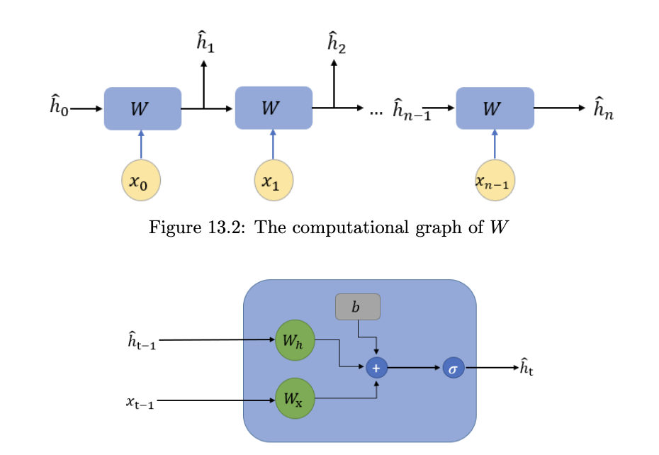
writing the RNN as a block matrix multiplication

and replace it by MLPs. Now, a box in the network becomes

Recall the structure of an RNN layer that takes in the input of the given time step and the hidden state:

The back propagation in RNN follows the same rule as any other neural networks,

Remark: Downsampling is not applicable in RNNs, because sequential inputs, unlike images or graphs, are not strongly connected at all regardless of the scenario.

Increasing Expressiveness in RNN

We can modify the transformation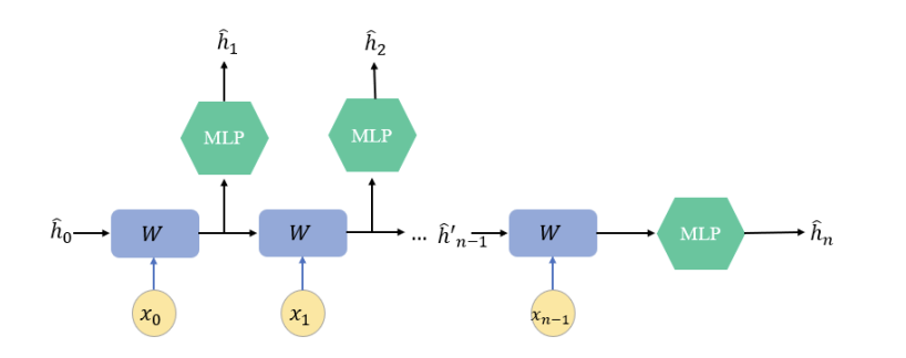, by either appending an MLP before returning each hidden state, or ifwere an MLP by adding the number of the dimensions in the output.

A more widely implemented method today is to compose the hidden states into more RNNs, thus providing both a better way of processing data as well as giving out a more intuitive explanation for weights. Namely, we can add horizontal layer.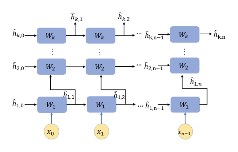

Dealing with Exploding Gradients

The most common way to deal with exploding gradients is to use saturating activation functions, which have a small gradient when the input is large. In other words, we are replacing ReLU with a function such as tanh or sigmoid.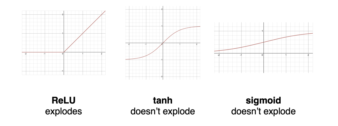

Gradient clipping is a standard technique to deal with exploding gradients in any kind of neural network.This requires simply clipping the gradients if they get above a certain value.
In the case of RNNs, this will stop the gradient from exploding, but it may have unintended consequences because it will distort the “shape” on which gradient descent moves. Therefore, historically, people use tanh/sigmoid for RNNs, and gradient clipping can be seen as a last resort.
Similar to CNN, we can also place a normalization layer between layers of an RNN, which helps deal with exploding gradients.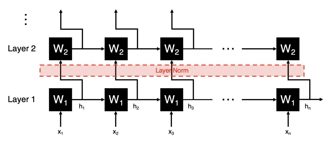

However, there is an issue because without the entire sequence available, normalization is impossible, since we don’t know all the values over which we want to normalize. One way to deal with this is to substitute the predicted effects of all other inputs we haven;t seen yet at test time to perform the normalization.
Another way to deal with this is mini layer norm,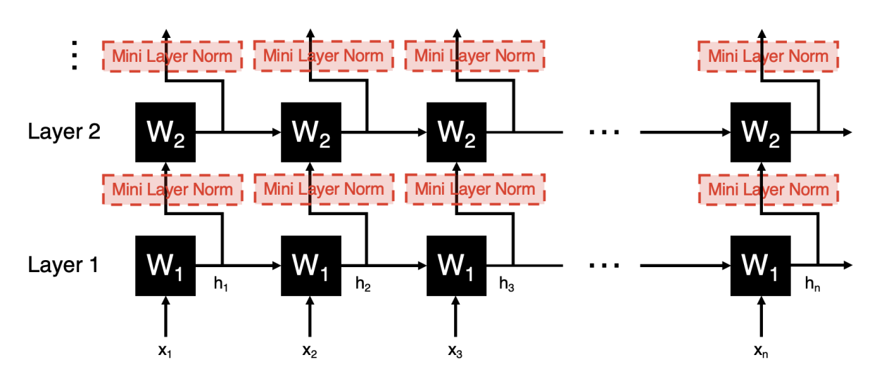

Mini vertical norm is the same as mini layer norm, except instead of normalizing a hidden state’s path to the next layer, it normalizes its path to the next sequence step.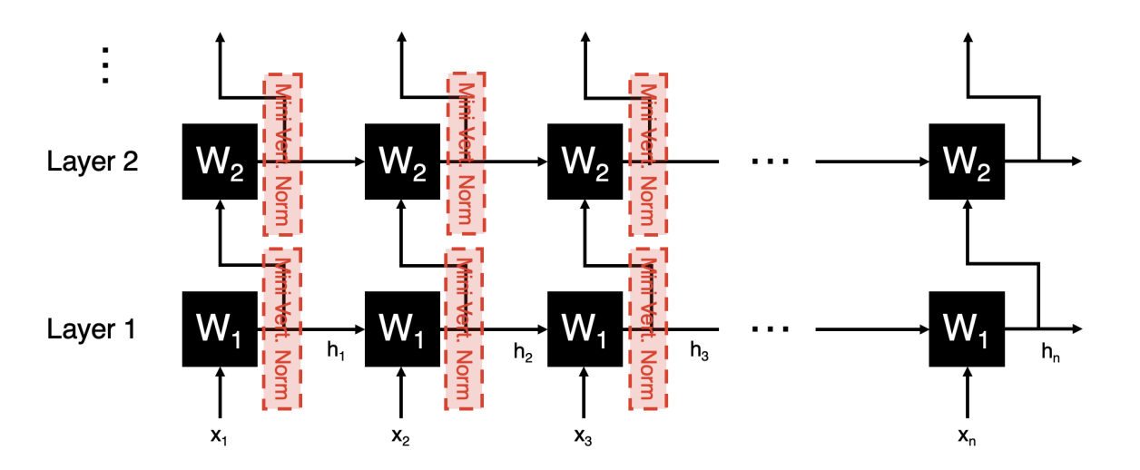

And please note that this vertical norm is not done in practice. Because there is no issue with computation, it is just not practical or desired to mix the effect of different learned filters.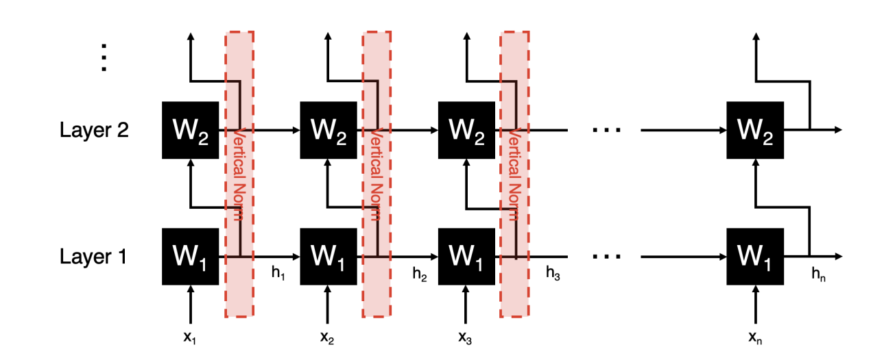

And for batch norm, this is possibe, but not usually done. Because it is more difficult to implement than other forms of normalization because sequences from different samples could have different lengths.

Dealing with Dying Gradients

We can apply the same thing like residual blocks into RNNs as well. The picture below shows vertical skips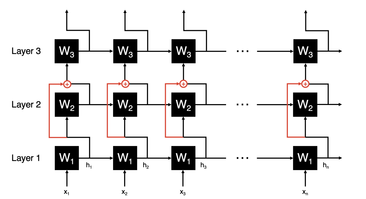

The picture below shows horizontal skips. It is true mathematically and helps with dying gradients, but it may change the inductive bias of the RNN.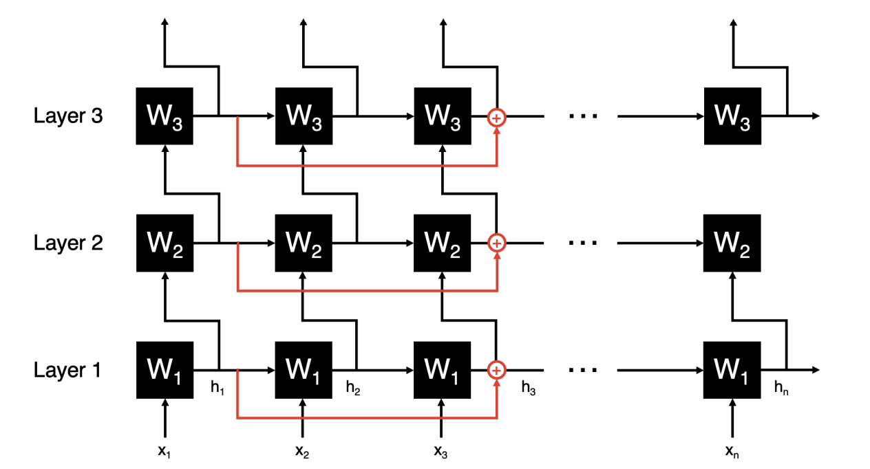

With RNNs, we typically want the learned weights to act primarily locally (in other words, learn mostly based on the input they directly receive at that sequence step). However, horizontal skips weaken this locality by bringing in an input from earlier in the sequence that will be less “dead” than the gradient coming from the sequence step directly previous. Put concisely, horizontal skips mean less favoring of local information (inputs nearby in sequence position).
Is this a bad thing? It depends on the application. If it relies heavily on local data (short-term dependence), we would need a lot more data to force the RNN to look locally instead of using gradients from the past. If it requires more long-term dependence, then we are okay.

Dealing with multi-scale Information(LSTM) Optional

Information can be gleaned at different levels of precision(e.g. sentence level, phrase level.) This presents some challenges:1. Context in the data is long-lived (e.g. a full sentence), but can shift suddenly (e.g. that sentence ends and a new one starts). 2. Details that the RNN is looking for evolve and mix at different points in the sequence.

Homeworks

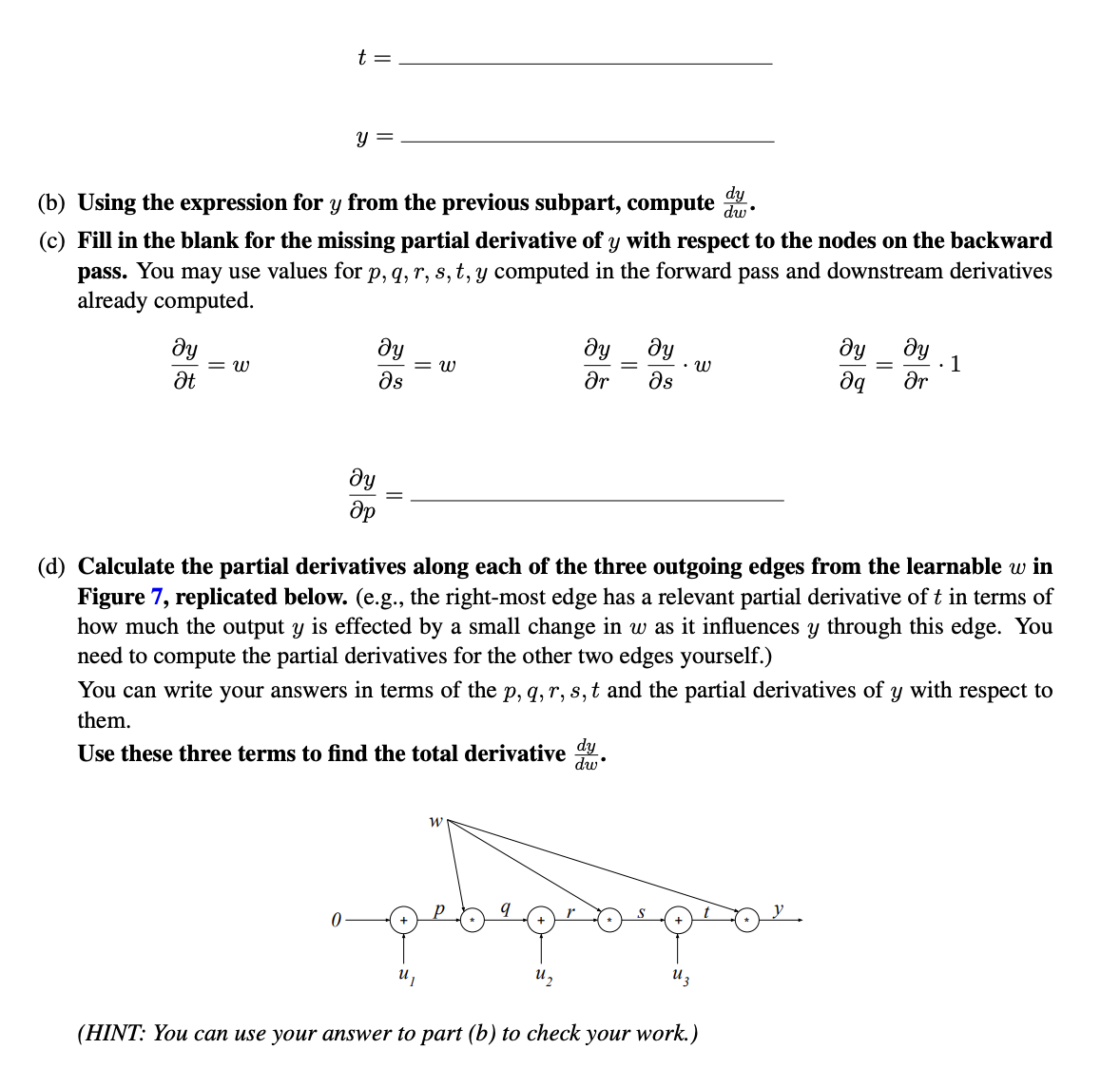
Backprop through a Simple RNN

Considering the following 1D RNN with no nonlinearities. The formula is given by: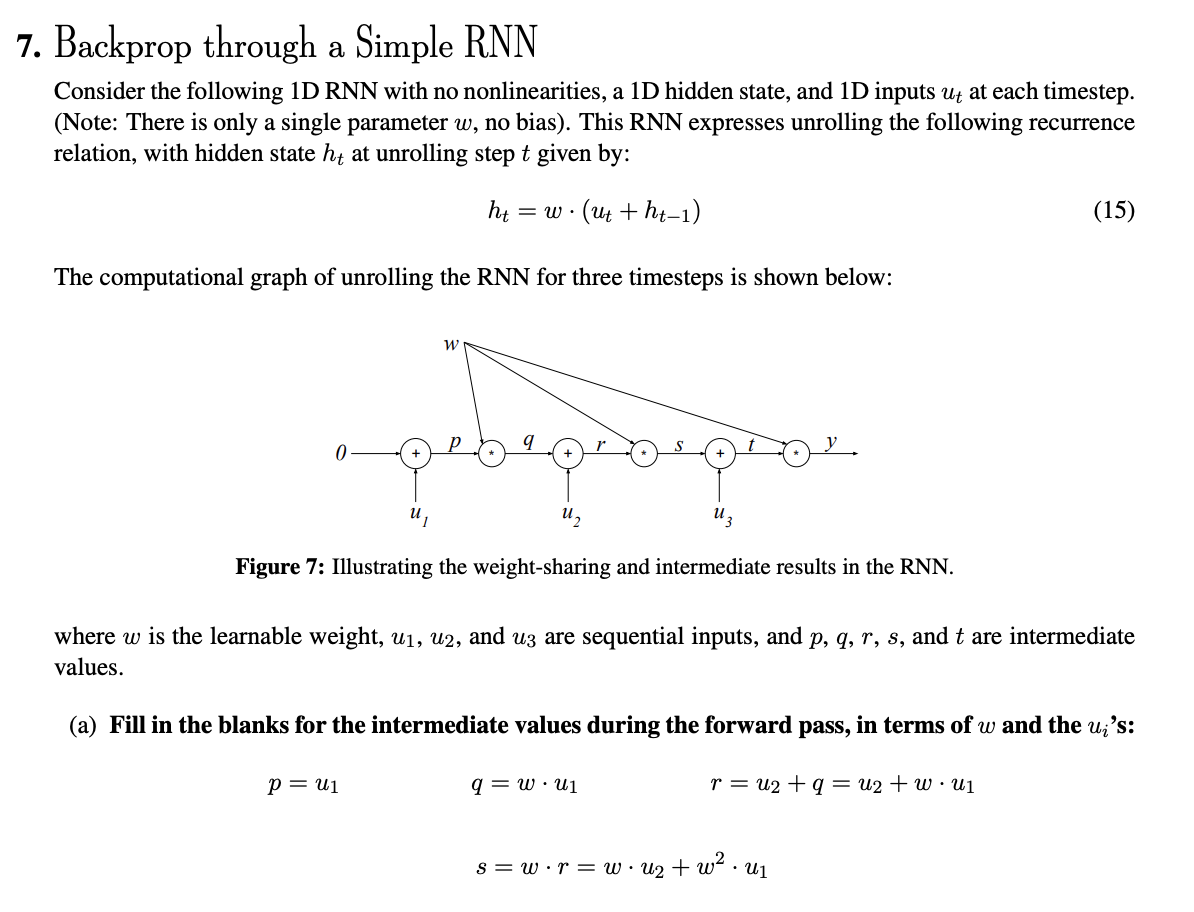


Ans:

Discussion

Seq-to-Seq Problems

Contents

The goal is to map an input sequence of data to an output sequence.(e.g. predicting, generating a sequence). It’s natural to consider RNN for seq-to-seq problems because RNNs are known to be useful using RNNs for seq-to-seq problems.

Machine Translation Example(Challenges)

There are potential challenges in RNN when utilizing it into machine translation tasks: 1. sequential processing process sequences one element at a time, which can result in slow computation for long sentences. 2. RNNs have a limited context window, which makes it difficult to capture relationships between words and phrases in longer sentences. 3. the order of the words in the source and target might be different, making it challenging for RNNs to learn correct alignment.

Encoder-Decoder Architecture

Each word is inputted into the encoder blocls sequentially and each block outputs a hidden state. Each block shares the same weight.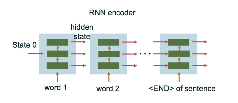

Decoder takes the input representation and generates the output sequence one element at a time. This allows the RNN decoder to capture dependencies and relationships between elements in the output sequence.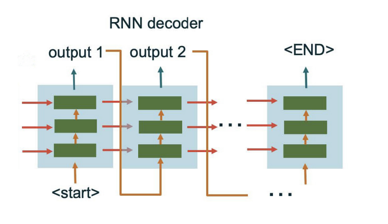

Teacher Forcing

While training decoders, in order to avoid accumulative errors, we use the ground-truth tokens as input for the next time step.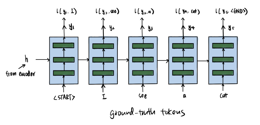

Auto-Regression

Autoregression is a technique that instead of using ground-truth tokens as input to the decoder at each time stamp, its tokens are generated by the decoder itself. Using noisy inputs helps the robustness of the model, which have a result ithat when received an imperfect token, the after parts can still stay stable. What’s more, instead of over relying on clean data inputs, it helps better predictions when dealing with small errors.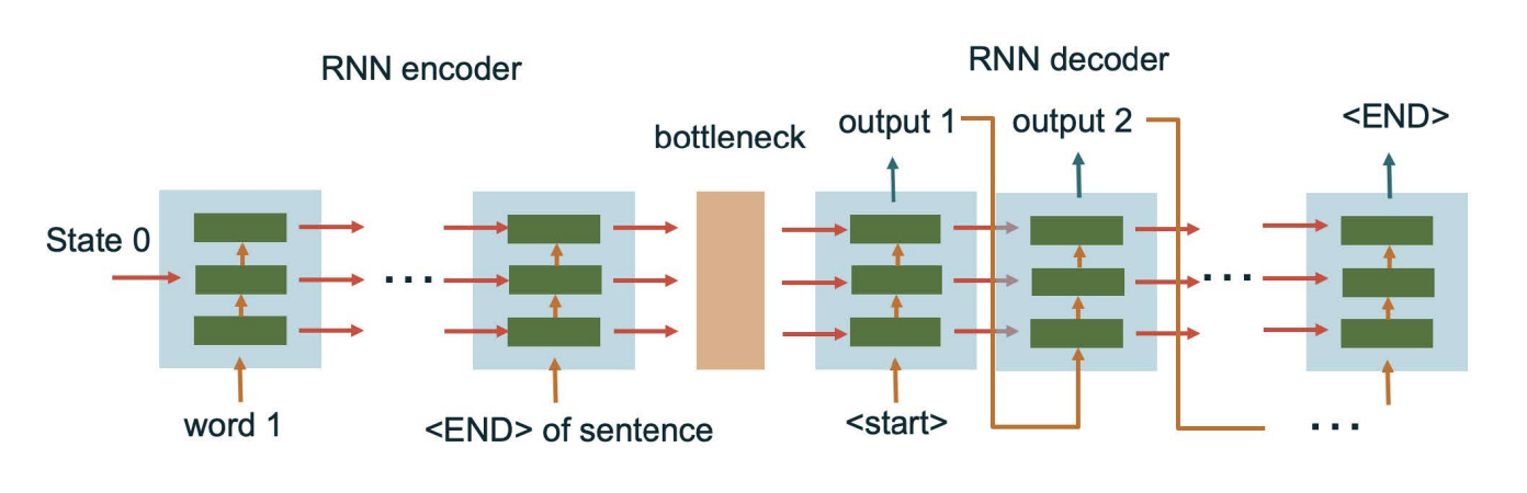

Cross-Entropy Loss for Language Problems

For sequence-to-sequence language generation tasks, the output data is discrete (e.g., words or characters), so cross-entropy loss is a very suitable choice. At each time step, the model produces a probability distribution over all possible tokens. We then use the one-hot representation of the ground-truth token to compute the loss:

During inference, if we use autoregression, we can no longer feed the full probability distribution as input to the next time step — instead, we must convert the distribution into a specific token. Common methods include:

1. Greedy decoding: Select the token with the highest probability
2. Sampling: Sample a token from the probability distribution
3. Beam search: Keep a small number of top candidate sequences and explore them in parallel

Homeworks

Discussions

Attention Mechanism

Contents

In language processing ,different languages have varying word orders, making the routing of information context-dependent. To address this issue, the goal is to add a “memory” to the existing Encoder-Decoder architecture that allows the input information to be stored and retrieved at the decoder. This allows the decoder has access to the right piece of information for every position, and facilitating the generation of high-quality output.

Queries-Keys-Values

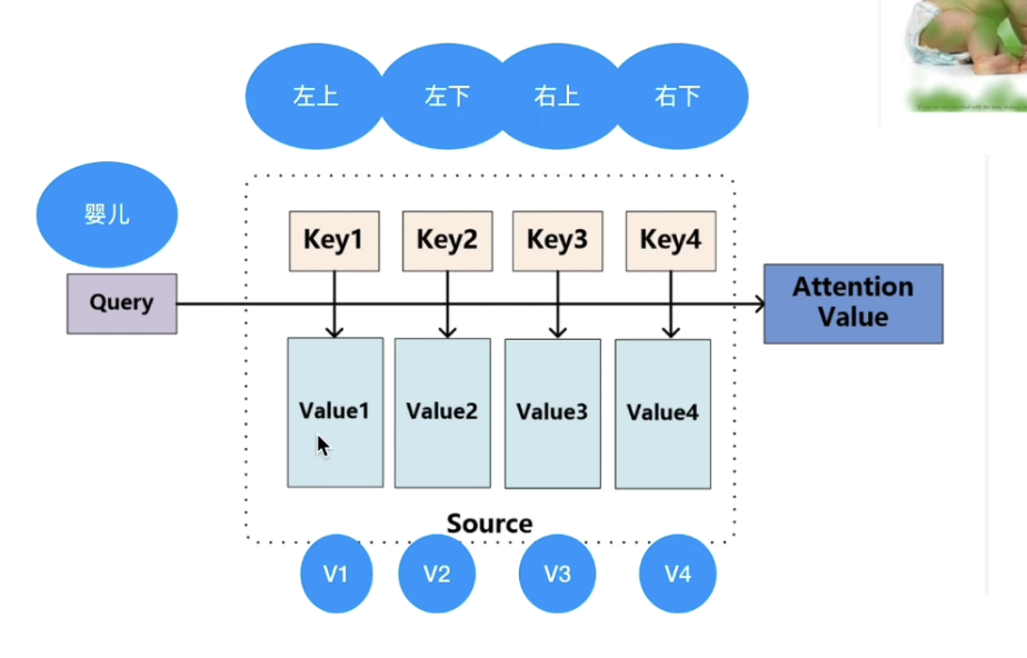
Unlike the traditional hash table, our query may not always match to keys in the hash table, so we need to design a differentiable hash table which not only can get an appropriate forward value, but also backpropagate to make it work while training.

Great Ideas in Attention

Idead(-1):look for an exact match for query and key and return a value
This doesn’t works since we always fail to get the return value because we don’t have the exact matching keys and queries. Additionally, we are unable to calculate the gradient using back-propagations since we won’t get any matches.
Idea(0): scan for the closest match for query to key in the hash table and return the value
we can search for a value now. But we are using the similarity between query and key, which means small changes to the query or the key will result in the same output, and the gradient will be 0 as well.
Idea(1):Scan for the closest matches of query to the keys. Then return a weighted average of the values.
In this way, attention can be thought of as “queryable pooling”, because keys and query values are also learnable parameters, but there are no learnable weights in the attention mechanism itself.
Picture below shows the attention mechanism in RNNs.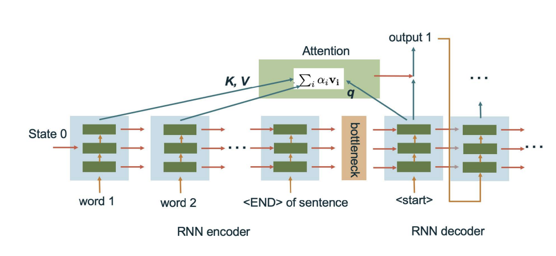

In this way, we have


Here, the similarity function can be softmax or some kernel-based methods. In attention, we will use the normalized inner product,

where d is the dimensions of q and k.(Here according to the central limit theorem, the product has a standard deviation that is proportional to the square root of the number of variables being added together. So normalizing by dividing the root of the dimension keeps the score within a reasonable range).
After that, we use softmax to compute the weights:

To get the answer, we can simply say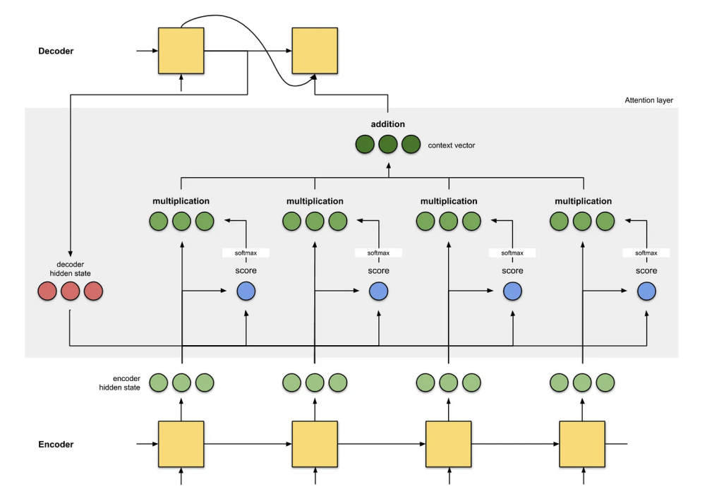

Cross-Attention and Self-Attention

If keys and values are obtained from the encoder, we call the attention layer Cross Attention. The key
and the value can use the same information as the input (like layer output / input etc.), but be generated
through different attention layers, so that they can focus on different parts of the info. If the key and the
value are from the decoder, we call it Self Attention. The benefit of this includes creating more routes to
prevent the gradient from dying. Note that in this way the key and the value must be causal, which means
they can only depend on the previous or current timestep. If time is current, only layers below can be seen
as the input. In a word, only the input side of the decoder can be used here.
In Cross Attention, there are two ways for the gradients to go backwards: One through the hidden states
through the RNN encoder, and the other through the attention mechanism and the key / value to the
encoder. The hidden-state route can keep track of the time info (e.g. what’s the last word input?), while the
attention is normally unordered across input subscript i. However, we can also add time to the attention
input directly, which is called positional encoding.

Homeworks

Kernelized Linear Attention(Part II)

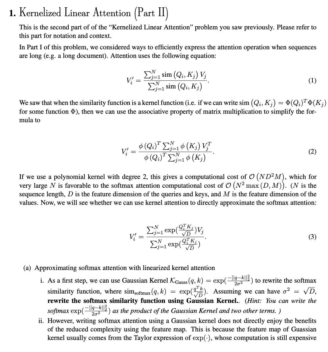
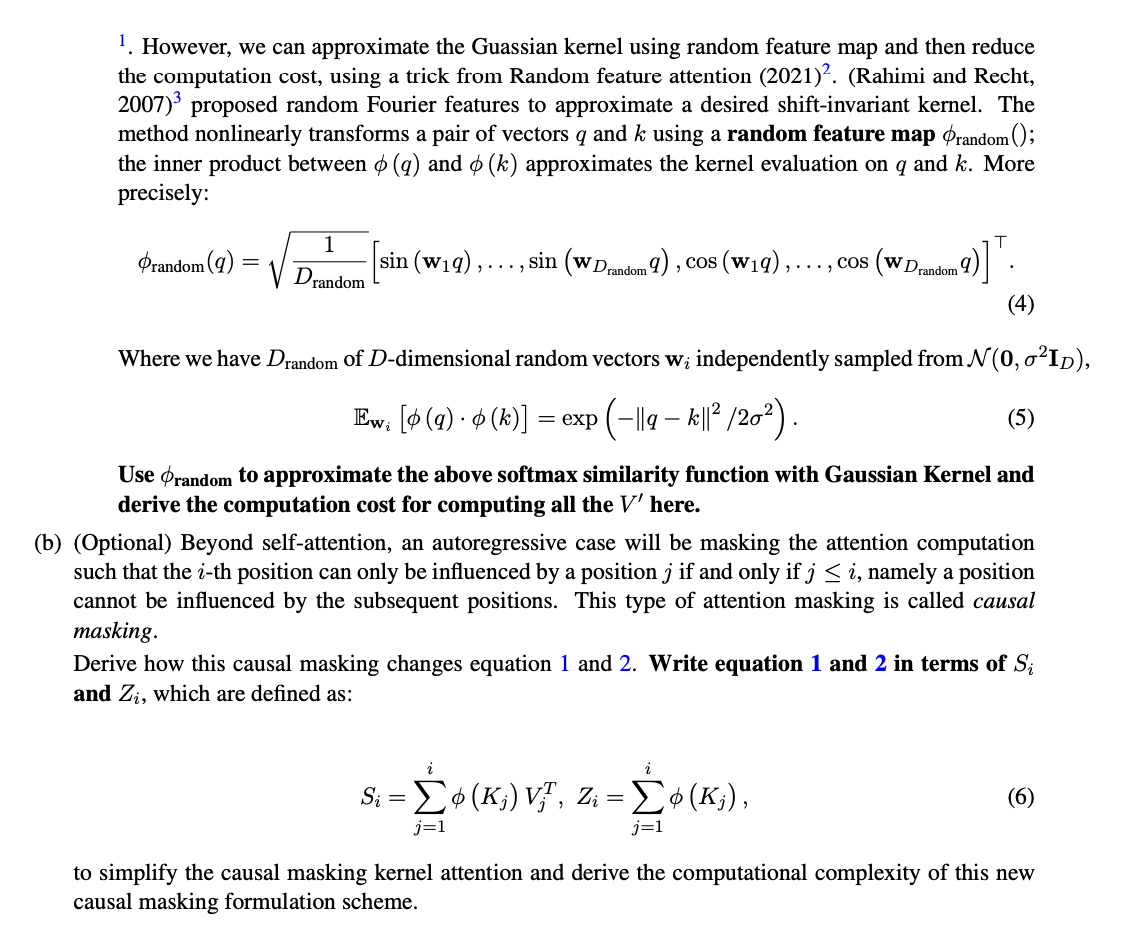
Ans:

Note thatandcan be computed byin constant time hence making the computational complexity of linear transformers with causal masking linear with respect to the sequence length.

Discussions

Self-supervision

Contents

Homeworks

Discussions

Transformer

Contents

Positional Encoding

Positional Encoding solves the problem that how to add time to the input vector.
Just increment a counter. Like mark the first place 1, the second place 2, etc. However, the number will becomes super large like 1000 fir the 1000th place. And it will cause an unbalanced encoding as the later places would be shining in the model.
Normalized counter. We set the largest step as 1 and the smallest number as 0. In this way, like for 1000, the difference between each step would be very tiny: just 0.001.
Use circular time. We have

In this way, the norm of the positional encoding is always 1. However, the difference between two steps would still be very tiny when w goes. However, ifis super small, the difference between two steps are still tiny, which means positional codes between two steps almost overlap and lost the ability for small-scale clarification.
Use an ordered list to store the key and the value instead of using unordered dictionar.

Homeworks

Discussions

Fine-tuning

Contents

Fine-tuning

Transformer and its training are very hungry for training data, as they have fewer assumption to data structures like CNN and RNN, so they have a much weaker inductive bias. One way to solve this is take advantage of unlabeled data like self-supervision. Another way is amortization across tasks. In practice, the transformer is pre-trained on some tasks and possibly by self-supervision, then do the adjustment(fine-tuning) for the task we specifically care about. The basic method is adding a new head as follows. We remove the old head, add a new head with random initialization and then train new head on rask-specific data, while freezing the rest of the net.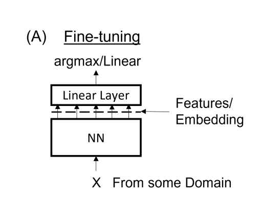

One way to think about this is that the last linear layer is the embedding of the learned features. We can choose anywhere along the newral network as the end of the embedding and remove the following structure as the old head.

Linear-Probing

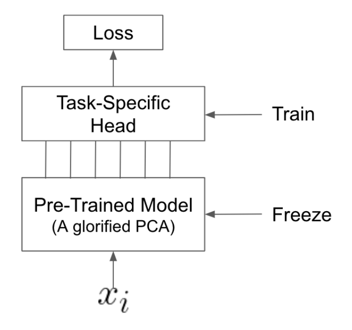
Classic way is to treat the pre-trained model as a feature extractor. We just train the head, freezing all the weight outside of those in the task-specific head.
Ways of generating features:1. generate features from the output of the penultimate layer; 2. use outputs from previous layers; 3. average the outputs of various layers together.

Full Fine-Tuning

Treat the pre-trained model as a good starting point as initialization. However, even if we train everything together, we still need to initialize the head. Here are several ways:
Approach #1: random initialization of the task specific head and begin the fine-tuning process. But it may send bad gradients through to the pre=trained model, potentially causing harmful changes to the pre-trained weights.
Approach #2: first random initialization and only train head, then train all the remaining and do full fine-tuning.
Classic method is faster and have lower requirement to the memory needed, while full fine-tuning have a higher accuracy but requires larger memory.

Updating A Subset of Weights

We can improve the pre-trained model itself by increasing the size of the network, using more data, using better and cleaner data or more proxy tasks, meta-learning, etc.
More than that, we can do something between full fine-tuning and classic approaches. (like just update a subset of weights in the pre-trained model). There are possible ways to determine which subset to update:

1. Update a different set of weights as you go.(Similar to SGD, only update part of the informations.)
2. Selectively unfreezing the model top-down, like fine-tune top k layers. However, recent paper shows that unfreezing the bottom layers may also work when the training data and the actual data have different distributions.
3. Selectively unfreeze Attention. When we use transformer, if we have different context-dependence compared to original training task, we can choose to unfreeze the attention components.

LoRA

When we are doing fine-tuning, we are most likely be moving in a subset of directions, which will approximate a low-rank update anyways by moving the important parameters a lot and moving the less important parameters very little. In order to perform LoRA, we introduce factorizations to our parameters,

whereis amatrix,is frozen, andisparameters.
LoRA can be generalized to what people call adaptors. These are other small structures put inside the pre-trained model to be tuned, and keeping everything else frozen. One way to think about it is:

SVD is a sum of rank 1 updates, starting with the most important updates.

Quantized Model

It’s a method used for compression. In compression, there are 2 things happening:1. transform the domain;2. use quantization to give appropriate precision to the places where there is action and nothing to places where there is no action. These models can be thought of as a glorified PCA. When using weight decay, the model will learn to favor specific directions. When performing full fine-tuning, we are locally working with a linearized version of the model around the neighborhood of the initialized weights. If a model has billions of parameters, it is most likely not having an equal amount of motion along all the different weight directions. There are likely some
directions that are more important than others.

Homeworks

Discussions

Embedding

Contents

GPT-Style Embedding

GPT-style is the self-supervise or auto-complete by next word/token prediction like the system-id style.
For language problems, we wish to get vectors from the text, which is called the problem of tokenizaiton and token embedding. This is done by parsing the input string into segments of tokens and followed by a look-up table that could be tuned/learned.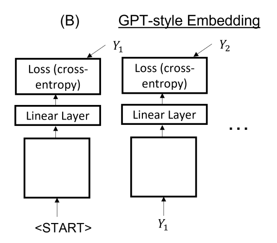

GPT-style embedding starts with <START> and outputs with a loss(cross entropy) between the first prediction and, then the network hasas input and predict the next. One benefit is that all the text could be used as the training data to do the next token prediction. The underlying lower dimensional structure or the embedding of language is presumably learned after training. The attributes of language are distilled from the autocomplete (next token prediction). One comment is that way more features than the training data may be obtained after this but that should be okay in our context. We may assume
the regularization works.

BERT-Style Embedding

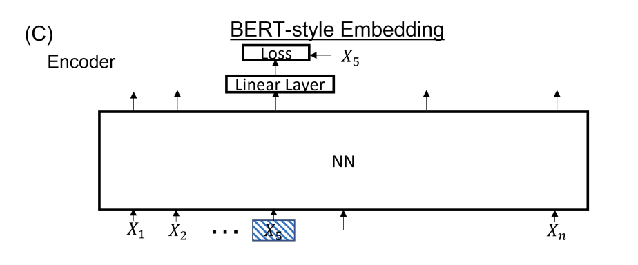
BERT Style does the data augmentation, such as the noisy and masked auto-endoding we have learned. Some fractions of the input are masked and the task is to reconstruct the embedding.(likehere), the input likecould be replaced with the mask which is a real vector.

Tokenization

Tokenization is necessary because textual information is given as sequence of strings from a discrete alphabet. There are 2 steps:1. parse the strings to a sequence of tokens. 2. map those tokens into vectors.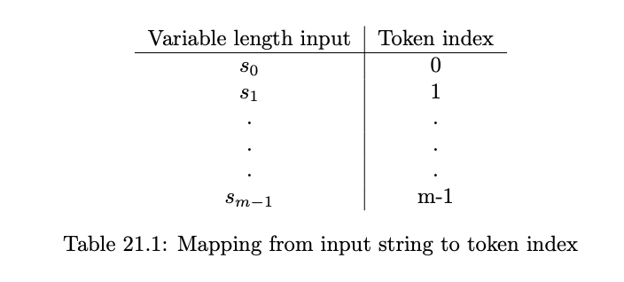

A natural way is to use letters of the alphabet as tokens, but the single letter is not a meaningful token. If we could have each token represent a meaningful unit instead, we effectively do this work for the model.We do that via a lookup table, where each of the m possible inputs is mapped to an index. And we want to ensure prefix freeness(i.e. no string is the prefix of another, so that there will be no ambiguity between “a” and “an”.)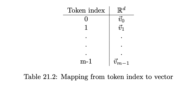

The we have the token as an index, we map those tokens to vectors.
Mapping vectors is easy, but the look-up table here in not a linear map, like the left column is discrete strings and cannot be calculated by gradient passing. One way to contruct such a linear map Byte Pair Encoding, which is similar to huffman encoding. The intuition is that occur commonly together do so because they represent a semantically meaningful unit.
Note that tokenization is done before training our model. Usually we just use the current tokenizers like OpenAI’s tiktoken.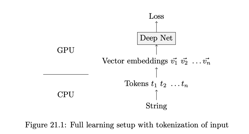

Word2Vec

We achieve this in the following way:

1. Randomly initialize two vectorsandfor each word.

2. Useto measure a score foras a likely neighbor for.

3. Train using “logistic loss style” loss, i.e.
   
   with randomly selected word. We comparewith positive examples that are its neighbors and random negative examples. We need to train with both positive and negative examples in order for the vectors to not all be, which would minimize the inner product between all vectors.

4. Use the average ofandas the final embedding.

BERT

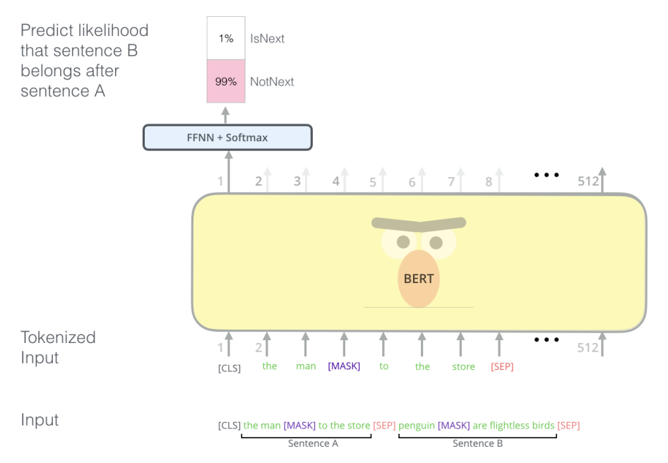
BERT is an encoder-style transformer, which means self-attention is not causal. Text input is first transformed into a vector(with learnable parameters) and concatenated to a positional embedding(without learnable parameters). The core model is composed of a stack of attention blocks with serial (or parallel) interconnections to NLP. At the end is a task-specific MLP that maps the embedding to scores for each token.
BERT is originally pre-trained on 2 tasks: one is masked denoising(predict the masked words), and one is changing the sentence order(predict if the order of two sentence is changed or not).
Two ways we utilizing BERT might be feature extraction and fine-tuning. Feature extractors. Treat the embeddings of the language model as a feature extractor and use any combination of the activations as an input to a separate model. While you could just use the penultimate layer, you could also use the last N layers and concatenate or average them. Selecting a subset of features becomes its own hyperparameter search.
Fine-tuning. Use BERT as a building block. Replace the task head (in this context, the head refers to the MLP fine-tuned to a specific task) with a new MLP. Fine-tuning can apply to just the final layer or to the entire model, but fine-tuning the entire model can actually degrade performance. This is because if the final layer’s weights are poor, the backpropagated weight updates may also be noisy and suboptimal. The present best practice is to freeze the pre-trained model first, and then train
everything.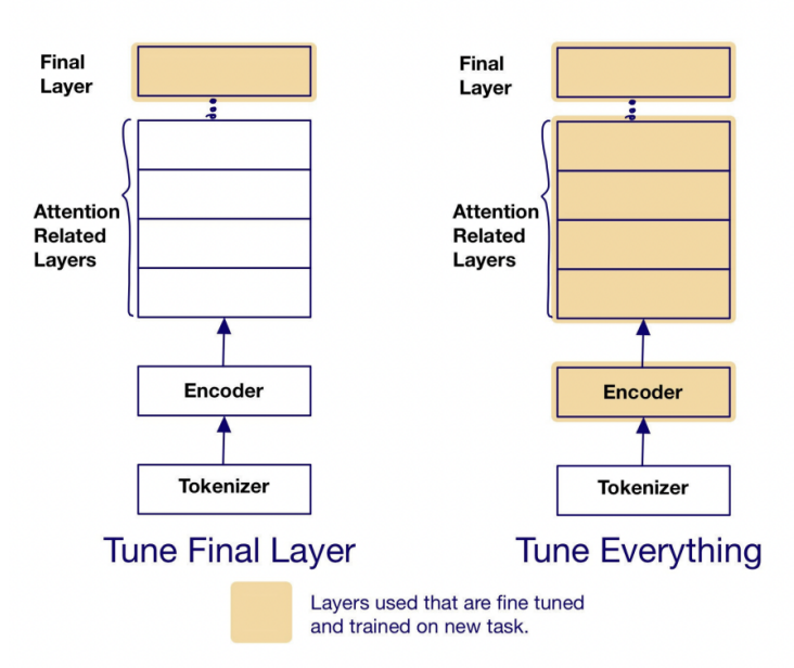

Homeworks

Discussions

Prompting

Contents

GPT-Style Models

GPT-style moels are trained on the task of auto-complete(next token prediction).
Zero-shot learning is an attempt to learn a task from no previous examples.(eg: prompt: the capital of france is. model returns: paris). In this example. the sentence generated from the following template

The entire pipeline with a blackbox GPT model can be seen below: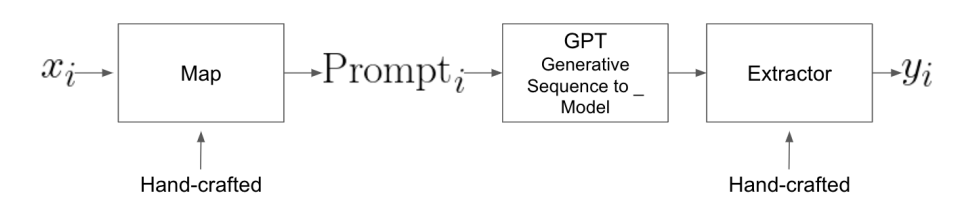

The area of generating prompts to solve specific tasks is generally known as prompt engineering.

Few-shot Learning

Few-shot Learning is an idea that provide the model some, but not much training data for the task through the prompt itself. The hope is that additional context will direct the model to provide better answers. Ex: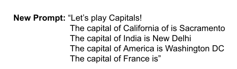

While the performance of few-shot learning is better than that of zero-shot learning, the
performance is still not great. This may be driven by two issues.
First issue is that the tranining data is greater than the context length of the model, which results in the training data won’t fit in the prompt. We can split the data into k batches, then feed one batch at a time and treat output as a combination.(We treat the GPT as black-box, without any updating in the inner weights).
The second issue is that we provide prompts in human-speech through tokens, but the natural language of computers is vectors. To address this issue, we choose to allow the prompts themselves to learn via GD, which is called.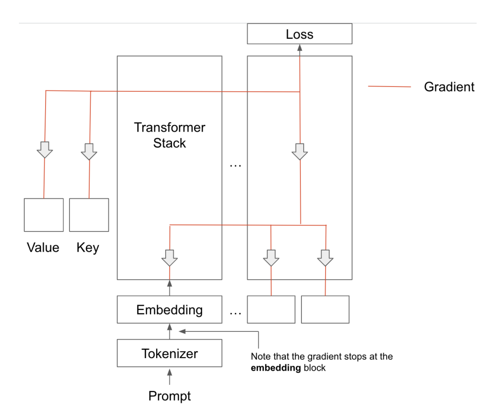

With soft-prompting:1. performance dramatically increases;2. only requires us to store a small number of parameters;3. memory usage is higher.

Homeworks

Discussions

Catastrophic Forgetting

Contents

What is CF?

When a model learns something new, it can forget something it already knows. This phenomenon can be viewed as both a feature and a bug, and here we treated it as catastrophic forgetting as a bug.(like we trained on recognizing handwritten 1, but when we then train on 2s, then both of the loss of 1 and 2 will increase).
Approaches for training on multiple tasks:1.freezing the model;2.linear probing strategy;3.soft prompt before pre-trained model;4.low-rank adapter.

Homeworks

Discussions

Knowledge Distillation

Contents

Homeworks

Discussions

Meta Learning

Contents

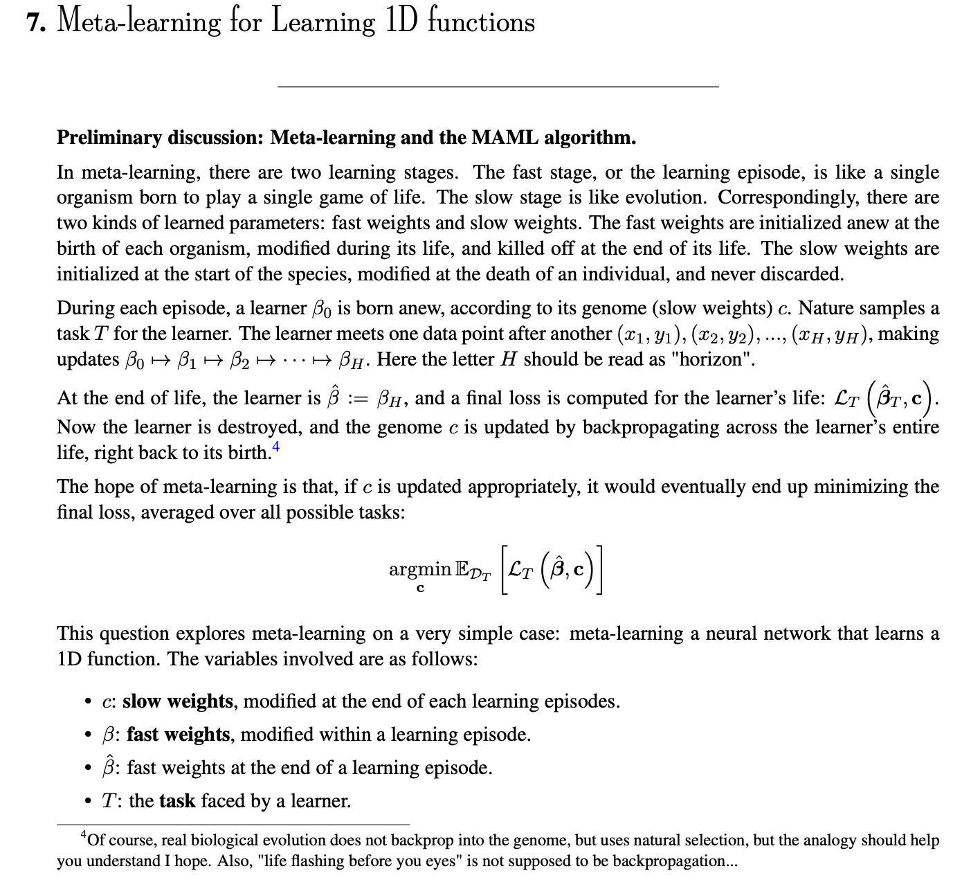
Idea of Meta-Learning

In meta-learning, fine-tuning is central (“on a task you can see”) as meta-learning means to learn how to learn. In practice, this means “we want to be trained so that we are good at being fine-tunable”.
Note: this is a distinction from “post-train” fine-tuning where the aim is to modify parameters after the main training is done. Now, the fine-tuning happens as we train since we know we are going to fine-tune anyways. This saves time and will in most cases produce better models.
The distinction here is that latter perspective treats fine-tuning simply as an interesting emergent property, while the meta-learning perspective considers optimizing fine-tuning as we train the model. So, this leads to the question of how to do this in practice.
When fine‑tuning with very little data, the model’s updates concentrate along a handful of dominant directions—the top singular vectors of its locally linearized input–Jacobian. If two tasks share these principal directions, gradient steps for the new task will overwrite the weights needed for the old task, causing catastrophic forgetting. Conversely, if each task’s dominant directions are orthogonal, fine‑tuning on one task induces negligible perturbation along the other task’s directions and thus preserves prior knowledge.

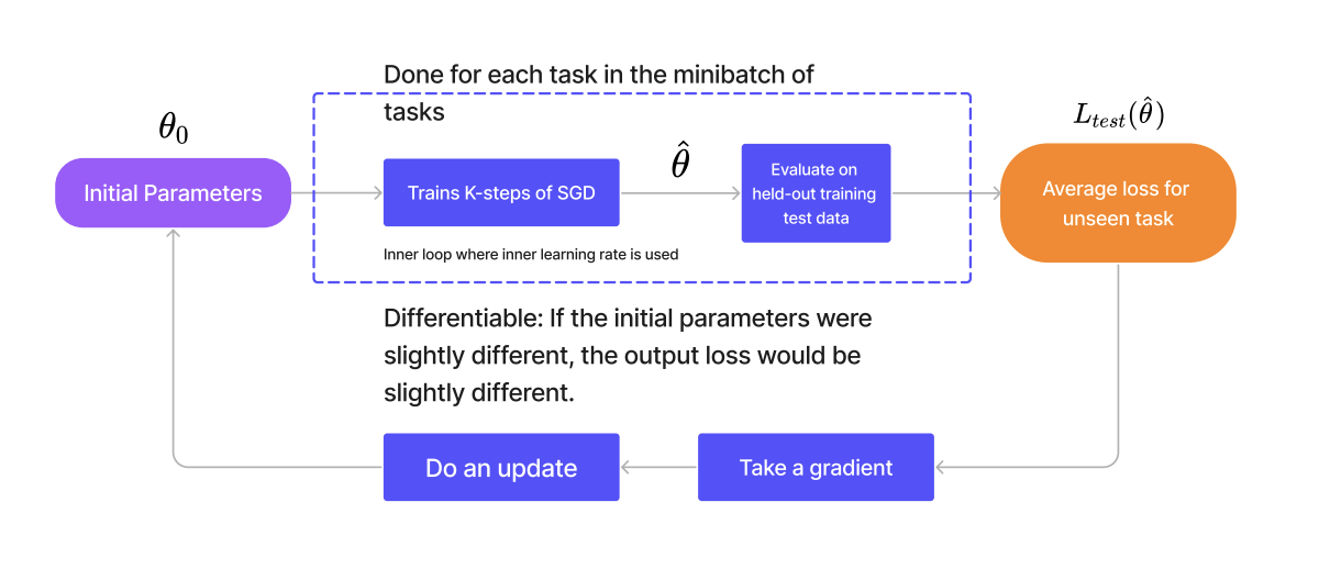
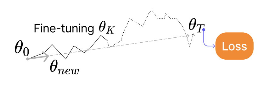
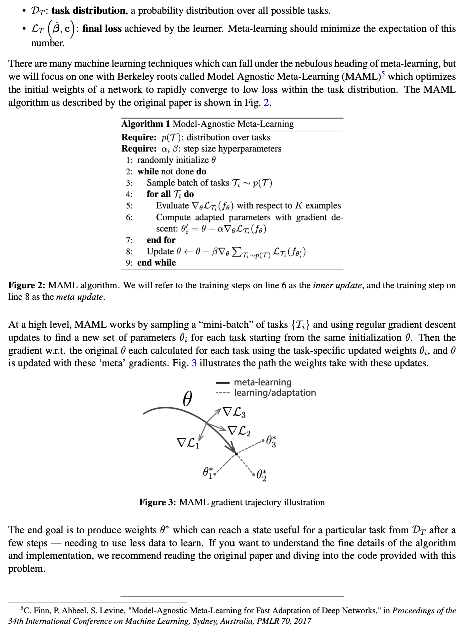
MAML

1. Assume we havetasks (Task, Task, …, Task), each with its own training and validation data, whereindexes the task andthe sample.

2. 
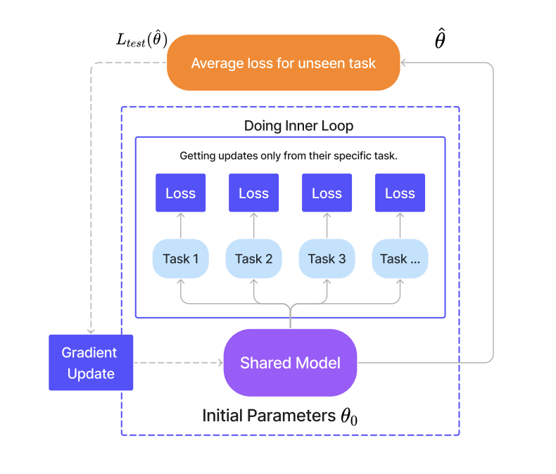
   For each task, starting from the shared initialization, performsteps of gradient descent on the task’s training loss to obtain task‑specific parameters:

3. 
   Evaluate eachon its validation set, sum the validation losses, and update the initializationvia gradient descent:

4. 
   MAML uses only standard gradient updates, making it compatible with any differentiable model—be it CNNs, RNNs, Transformers, or reinforcement‑learning policies.
   
   

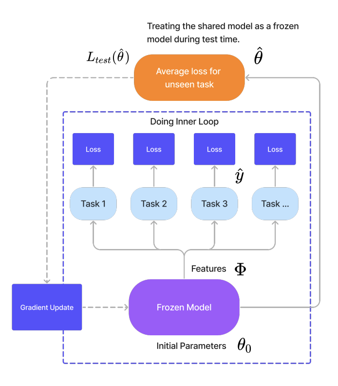
Semi-Frozen

In the semi‑frozen approach, we begin by unfreezing the shared, pre‑trained backbone during multi‑task training so that it can accumulate updates across all tasks and converge to an optimal initialization. Once this “best” checkpoint is reached, we freeze the backbone again at test time: for each new task, we restore the checkpoint, fine‑tune only the task‑specific components (or head), and leave the shared layers untouched. Whenever another task arrives, we simply reload the same checkpoint and repeat the local fine‑tuning. By combining an initial phase of full adaptability with a later phase of targeted, frozen‑backbone tuning, this method strikes a balance between the stability of self‑supervised pre‑training and the flexibility of task‑specific adaptation.

Subset Strategy

In the subset strategy, when a task’s full training set is too large to traverse in only K inner‐loop steps, we randomly sample a smaller subset of examples (e.g. 100 out of 1,000) and perform our SGD‐based fine‑tuning on just that mini‑batch. This lets us respect memory and compute limits while still giving the model a representative glimpse of the task. However, because we never see the task in its entirety during those K steps, we can’t fully measure how the initial initialization would behave on all data, and our “exploratory” updates become only a rough approximation of full fine‑tuning—making the algorithm practically resemble standard SGD more than true meta‑learning.

Reptile Strategy

In the Reptile strategy, instead of computing the full meta‑gradient, we simply take the difference between the fine‑tuned weights and the initialization () as a proxy for the update direction. After running K inner‑loop SGD steps on a sampled task to reach, we move the shared parameters slightly towardusing this vector. By repeating this across many tasks—and optionally unrollingsteps—we approximate the effect of second‑order gradients without ever forming or inverting a Hessian, thereby avoiding exploding gradients and greatly simplifying implementation.

Closed Form Strategy

In the closed‑form strategy, we treat the frozen shared backbone as a fixed feature extractor and train only lightweight, task‑specific heads (e.g. linear regression) by directly applying the closed‑form solution of a convex problem, such as least squares:. Because this analytic formula is differentiable, we can still backpropagate to compute gradients with respect to the initialization, all without performing iterative SGD steps. This both removes exploding‑gradient risk and drastically reduces computation and memory overhead, yielding a concise and reliable fine‑tuning mechanism tailored to each task.

Homeworks

Meta-Learning For Learning 1D Functions

Ans:

Discussions

Transfer Learning

Contents

Homeworks

Discussions

Generative Models

Contents

Homeworks

Discussions

Diffusion Models

Contents

Homeworks

Discussions