(CS182)Machine Learning Review

Scope of Final Exam

:
Bayes’ Decision Rule, Discriminant Functions
:
Maximum Likelihood Estimation, Bayesian Estimation, Paramatric Classification, Model Selection
:
Paramatric Classification Revisited
:
Multilayer Perceptrons
:
Hard-Margin SVM, Soft-Margin SVM, Kernel Extension
:
PCA, LDA
:
k-Means Clustering Algorithm, EM algorithm, Use of Clustering
:
Nonparametric Density Estimation, Nonparametric Classification
:
CNN, RNN
:
Voting, Boosting

Cross-Validation, Interval Estimation, Performance Evaluation

Preliminaries

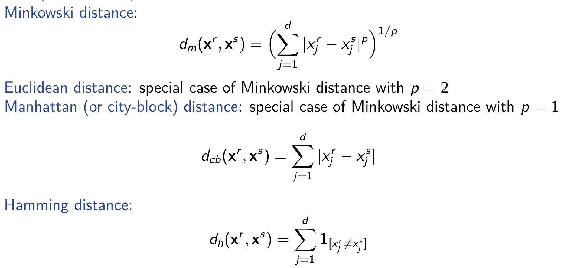
Distance Measures

Distance between instance

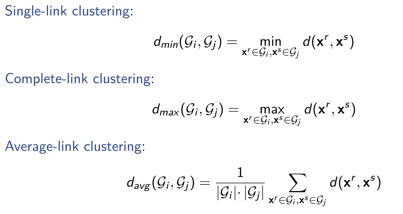
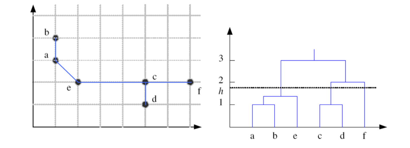
Distance between groups

Linear Algebra

Transpose

Matrixis orthogona ifand

Inverse

Gradient Vector

Positive Semidefinite Matrices

A symmetric matrixis said to be:
positive semidefinite:for all
positive definite:for all
indefinite: bothandare not positive semidefinite

Ifandis, with, thenis positive definite. If, thenis positive semidefinite.
A positive definite matrix can be “factored” as,whereis a nonsingular upper triangular matrix. One way to obtainis by Cholesky decomposition.

Eigendecomposition(Spectral Decomposition)

where Q is a squarematrix whose columns are the eigenvectors ofordered in terms of decreasing eigenvalues, andis a diagonalmatrix whose diagonal elements are the corresponding eigenvalues.
Ifis symmetric, its eigenvectors are mutually orthogonal and the eigenvalues are real. In this case, it can be written as

Singular Value Decomposition

Ifis, it can be written as

whereisand contains the orthonormal eigenvectors ofin its columns,isand contains the orthonormal eigenvectors ofin its columns, and thematrixcontains thesingular values,on its diagonals that are the square roots of the nonzero eigenvalues
of bothand; the rest ofis zero.

whereandare of different sizes but are both square and contain on
their diagonal and 0 elsewhere.

Optimization Primer

Lagrange multipliers can transfer a problem withvariables andconstraints to a problem that hasvariables and no constrains.
Standard foem problem:

Lagrangian

Assume we do not consider the constraints and obtain the optimal value in point, we have 3 situations.

For the first situation, the constrains is ignored and satiesfied automatically. For the second situation, we can obtain the answer by simply calculate the Lagrangian. For the third situation, we should discard the answer. And in conclusion, if, the problem can be transformed into a problem without constraint and if, we can use Lagrange multiplier. And in conclusion,

And we have

Above all, we can conclude the Karush-Kuhn-Tucker condition: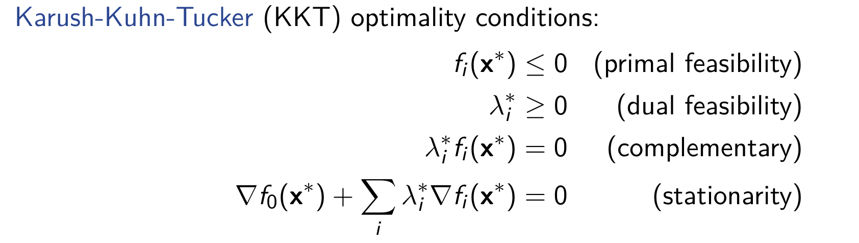

Bayesian Desicion Model

Parameter Estimation

Linear Discrimination

Multilayer Perceptions

Support Vector Machines

Hard-Margin Support Vector Machine

Definition of hyperplane

Definition of distance

If the sample point can be classified properly, we have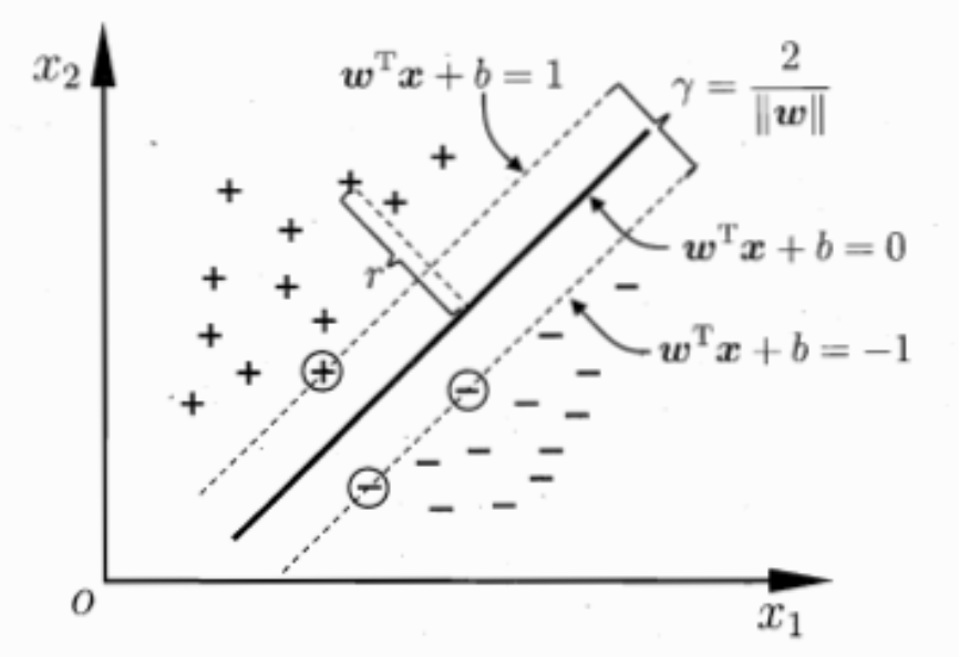

Nearest points to the hyperplane are called support vector, and the sum of distance of two support vectors to the hyperplane from different class is called margin

We want to maximize the distance, or equivalently, minimize, we have

Dual Problem

We have its lagrangian form

Calculate its derivative and we have

And we can have its dual form

It should satisfy KKT conditions

And if we havecalculated, we have

where its optimal will be

Soft-Margin Support Vector Machine

Relaxed seperation constriants

Primal optimization problem

Its lagrangian can be written as

Dual problem

And its KKT conditions are

kernel extension

Instead of defining a nonlinear model in the original (input) space, the problem is mapped to a new (feature) space by performing a nonlinear transformation using suitably chosen basis functions.

Similarly, we have

Its dual problem is

Since calculatingis difficult, we can use kernel trick to avoid this problem(calculate its value in original space)

And we can rewrite the dual problem as

And the answer is

Polynomial kernel:

where ( q ) is the degree.

E.g., when ( q = 2 ) and ( d = 2 ),

which corresponds to the inner product of the basis function

When ( q = 1 ), we have the linear kernel corresponding to the original formulation.

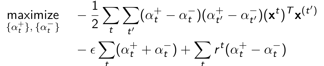
Support Vector Regression

Minimization Problem:

$$
\text{minimize}{\mathbf{w}, w_0} \quad \frac{1}{2} |\mathbf{w}|^2 + C \sum_t \left( |r^t - f(\mathbf{x}^t)| - \epsilon \right)+
$$

Primal optimization problem:

Lagrangian:

$$
\begin{aligned}
\mathcal{L}(\mathbf{w}, w_0, {\xi^+_t}, {\xi^-_t}, {\alpha^+_t}, {\alpha^-_t}, {\mu^+_t}, {\mu^-_t}) = \frac{1}{2} |\mathbf{w}|^2 + C \sum_t (\xi^+_t + \xi^-_t) \

\sum_t \alpha^+_t \left[ \epsilon + \xi^+_t - r^t + (\mathbf{w}^T \mathbf{x}^t + w_0) \right] \
\sum_t \alpha^-_t \left[ \epsilon + \xi^-_t + r^t - (\mathbf{w}^T \mathbf{x}^t + w_0) \right] \
\sum_t (\mu^+_t \xi^+_t + \mu^-_t \xi^-_t)
\end{aligned}
$$

Dual optimization problem:

Function Representation:

Dimentionally Reduction

Principal Component Analysis

We aim to fina a linear mapping from d-dimensional input space to k-dimensional with minimum information loss according to some criterion(k<<d)
We have the scalar projection ofon the directions.t.

we want to find the component that can make the sample points the most spread out, which simply can be achieved by maximize its variance,

And the goal of PCA will be

and we can do eigenvalue decomposition to covairencematrix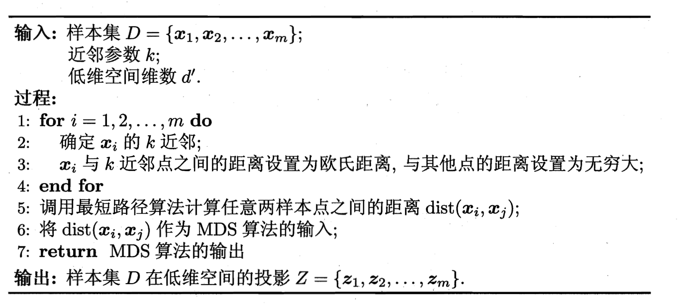, and sort the eigenvalue. The answer to PCA is the fronteigen vectors

And for choosing the detalied number of k, we can have a threshold,i.e..Then, we use this formula to choose the minimal,

Factor Analysis

The target of FA is opposite to that of PCA:
PCA (from x to z):

A (from z to x – generative model):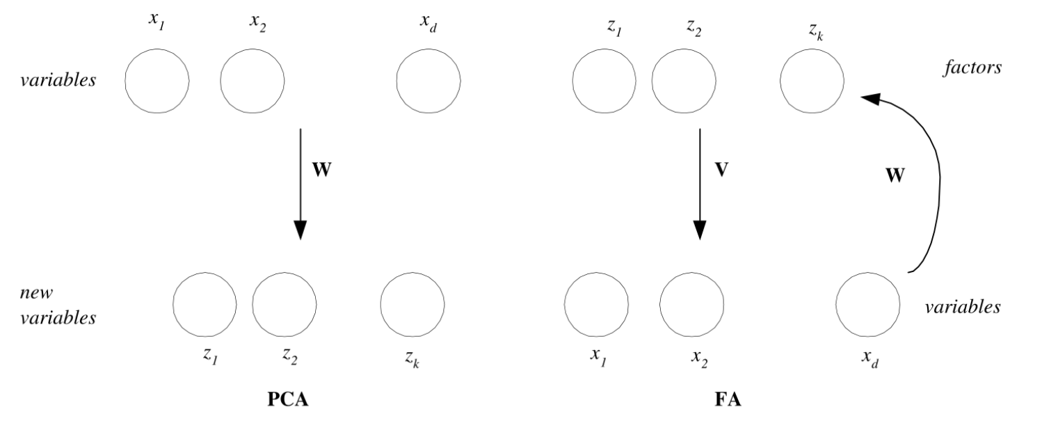

Multiple Dimensional Scaling

We want to embed the points in a lower-dimensional space (e.g., two-dimensional space) such that the pairwise Euclidean distances in this space are as close as possible to those in the original space.
Assuming m sample point in original space have a distance matrix, we aim at get representation of sample indimensional space, s.t.(disntance in-dimensional space equals that in original space)
Let,is the inner product of sample after dimensional reduction, we have

Centering of data to constrain the solution:

And it is obvious that the sum of the row and column ofis zero, then

Let’s have
$$dist_{i*}^2=\frac{1}{m} \sum_{j=1}^m dist_{ij}^2\quad dist_{j}^2=\frac{1}{m} \sum_{i=1}^m dist_{ij}^2 \quad dist_{i}^2=\frac{1}{m^2} \sum_{i=1}^m \sum_{j=1}^m dist_{ij}^2b_{ij}=\frac{1}{2} (b_{ii}+b_{jj}-dist_{ij}^2)=-\frac{1}{2}(dost_{ij}^2-dist_{i*}^2-dist_{j}^2+dist_{**}^2)B=V \Lambda V^T$$
And let $\Lambda_{}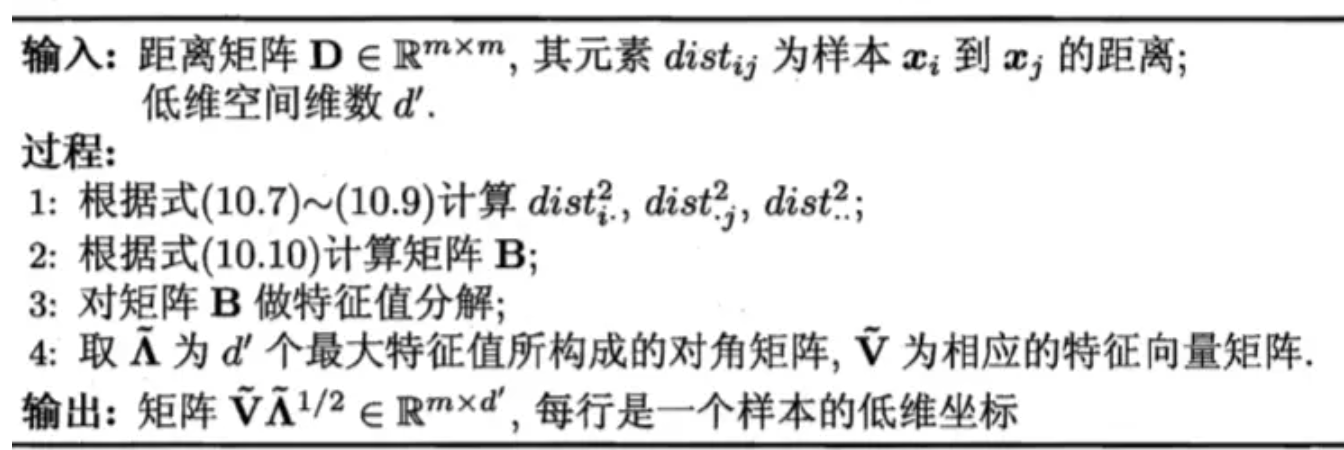d’V_{}$Z=\Lambda_{}^{1/2}V_{*}^T \in \mathbb{R}^{d’ \times m}$$

Linear Discriminant Analysis

Goal: the classes are well-separated after projecting to a low-dimensional space by
utilizing the label information (output information).
Letbe the set, mean vector, covariance matrix of-th sample set. We have the center of each class after projection, and sample covariance.
We want to minimize covariance between in-class covariance

Also, we want to maximize the distance between center of classes
$$ ||w^T \mu_0- w^T \mu_1||{2}^{2}J=\frac{||w^T \mu_0- w^T \mu_1||2^2}{w^T \Sigma_0 w+ w^T \Sigma_1 w}=\frac{w^T (\mu_0-\mu_1)(\mu_0-\mu_1)^T w}{w^T \Sigma_0 w+ w^T \Sigma_1 w}S_w=\Sigma_0+\Sigma_1=\sum{x\in X_0}(x-\mu_0)(x-\mu_0)^T+\sum{x\in X_1}(x-\mu_1(x-\mu_1)^T )S_b=(\mu_0-\mu_1)(\mu_0-\mu_1)^TJ=\frac{w^T S_b w}{w^T S_w w}min_w -w^T S_b w \quad s.t. \quad w^T S_w w=1\lambda(\mu_0-\mu_1)=S_b w= \lambda S_w w \Rightarrow w=S_w^{-1} (\mu_0-\mu_1)S_t=S_b+S_w=\sum_{i=1}^m (x_i-\mu)(x_i-\mu)^T, \quad S_w=\sum_{i=1}^N S_{w_i}, \quad S_b=S_t-S_w=\sum_{i=1}^N m_i(\mu_i-\mu)(\mu_i-\mu)^Tmax_w \frac{tr(W^T S_b W)}{W^T S_w W}$$
the solution is the eigen vector relevant to-th maximal non-zero eigenvalue of the matrix

Clustering and Mixture Models

Introduction

Mixture(density) model

=mixture components(clusters or groups)
=component densities
=mixture proportions (priors)

Gaussian Mixture Model(GMM)

parameters

K-Means Clustering Algorithm

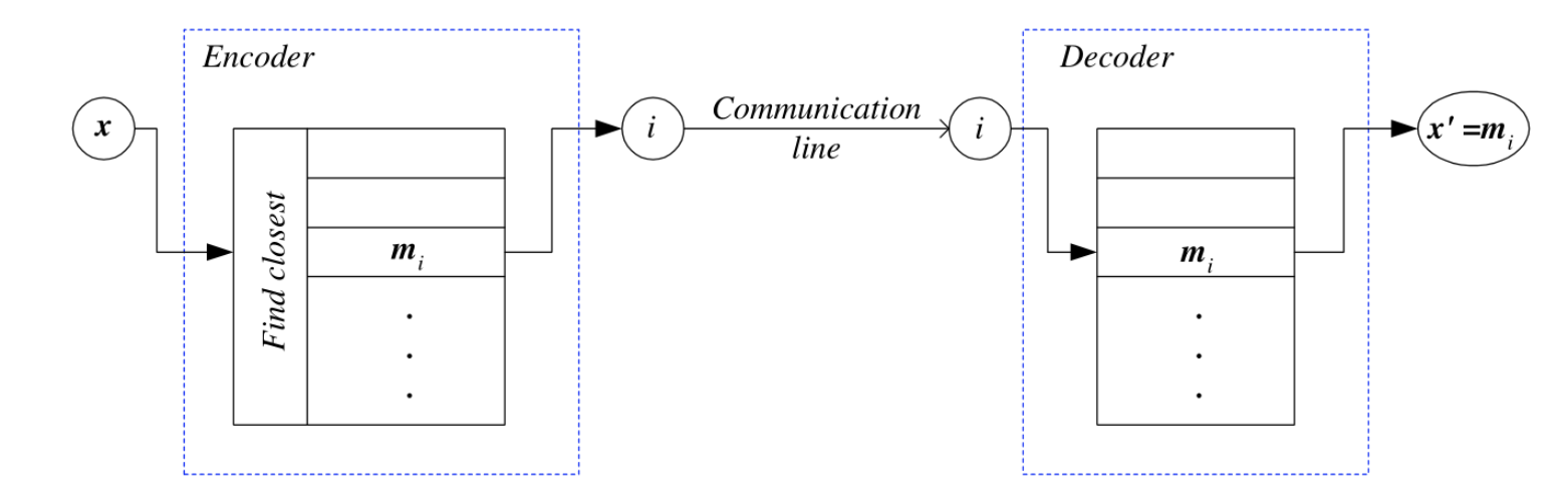
Encoding: from data pointto the indexpf a reference vector
Decoding: from an indexto the corresponding reference vector
Each data pointis represented by the indexof the nearest refernce vector:

Total recontruction error

where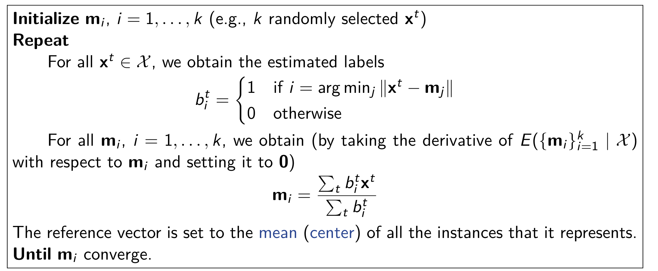
ifand 0 otherwise.

Expectation-Maximization Algorithm

For unobserved data, we can use EM to do estimation. We call this unobserved variables.
Letbe observed variables, andrepresent latent variable andbe model parameters, we have

Since Z is latent variable, it can not be optimized directly, we can calculate the expectation ofto maximize marginal likelihood for observed variable iteratively.

E-Step

Infer the distribution of latent variablesby current parameterand calculate its log likelihood for the expectation of

M-Step

Find parameterthat maximize expectation likelihood, namely

In one word, EM calculate global optimal by caulate expectation of current parameter and find the parameter that can maximize likelihood expectation.

Use of Clustering

Data Exploration

Like dimensionality reduction methods, clustering can be used for data exploration:
Dimensionality reduction methods: find correlations between features (and thus group features).
Clustering methods: find similarities between instances (and thus group instances).
Clustering allows knowledge extraction through:Number of clusters,Prior probabilities,Cluster parameters

Clustering as Preprocessing

After clustering, the estimated group labels may be seen as the dimensions of a new k-dimensional space.

Mixture of Mixtures in Classification

In classification, when each class is a mixture model composed of a number of
components, the whole density is a mixture of mixtures

withs

Hierarchical Clustering

Nonparametric Methods

Deep Learning Models

Deep Autoencoders

An autoencoder (AE) is a feedforward neural network for learning a compressed representation or latent representation (encoding) of the input data by learning to predict the input itself in the output.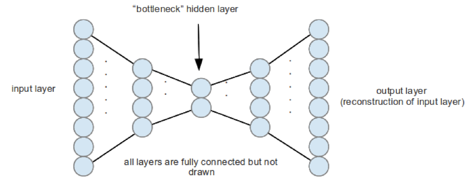

The hidden layer in the middle is constrained to be a narrow bottleneck (with
fewer units than the input and output layers) to ensure that the hidden units
capture the most relevant aspects of the data.

Stacked Denoised Autoendcoder

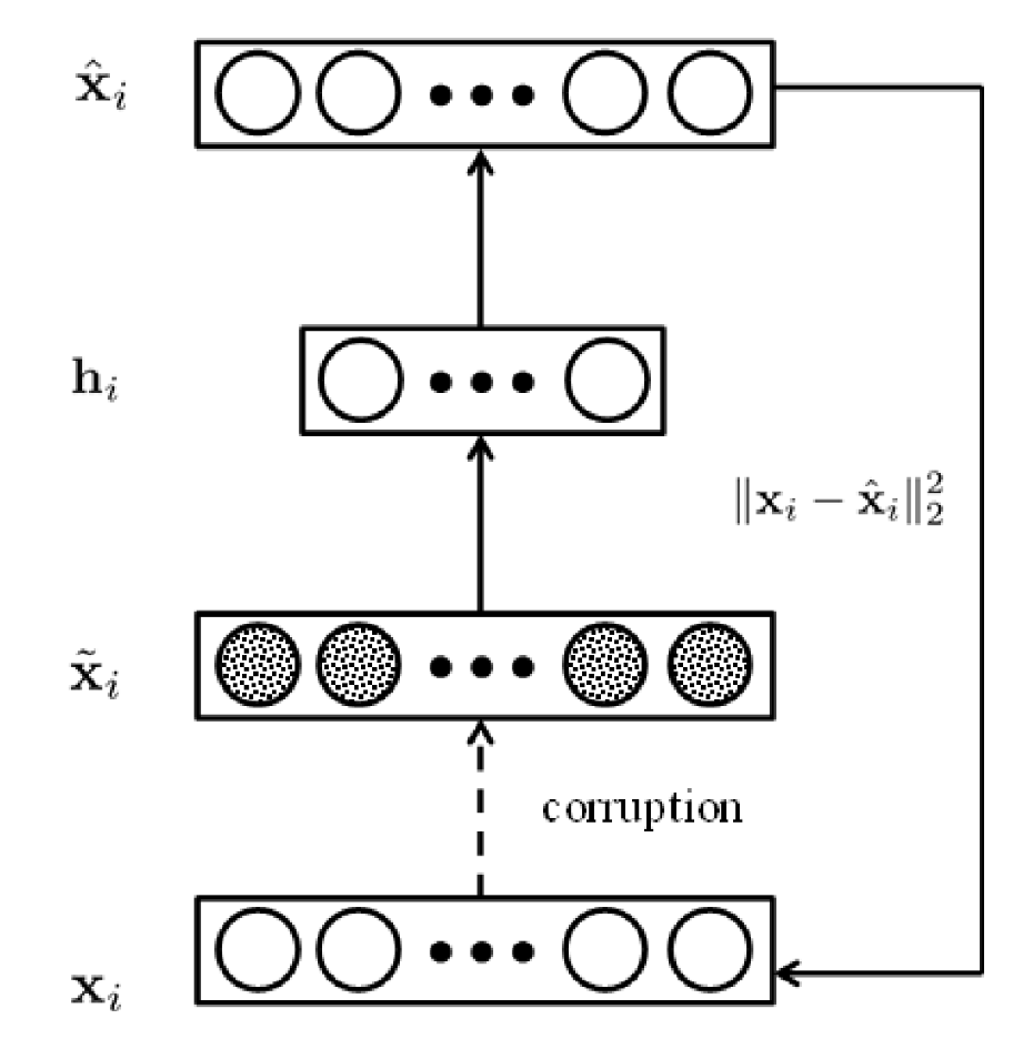
A denoising autoencoder solves the following (regularized) optimization problem:

$$\text{minimize}_{\mathbf{W}1, \mathbf{W}2, \mathbf{w}{01}, \mathbf{w}{02}} \quad \frac{1}{2} \sum_\ell | \mathbf{x}^\ell - \hat{\mathbf{x}}^\ell |_2^2 + \lambda \left( | \mathbf{W}_1 |_F^2 + | \mathbf{W}_2 |_F^2 \right)$$

where

$$\begin{aligned}
\mathbf{h}^\ell &= \sigma(\mathbf{W}1 \tilde{\mathbf{x}}^\ell + \mathbf{w}{01}) \
\hat{\mathbf{x}}^\ell &= \sigma(\mathbf{W}2 \mathbf{h}^\ell + \mathbf{w}{02})
\end{aligned}$$

Hereis a regularization parameter andis a matrix norm, called the Frobenius norm, which is defined as

$$| \mathbf{A} |F^2 = \sum{i,j} a_{ij}^2 \quad \text{where} \quad \mathbf{A} = [a_{ij}] \text{ is a matrix}$$
Stacked denoising autoencoders can be formed by stacking the denoising
autoencoders in a layer-wise manner like deep autoencoders with the same
pretraining, unrolling, and fine-tuning steps.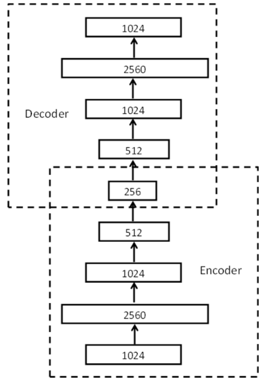

Convolutional Neural Networks

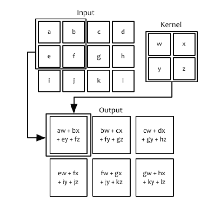
Dropout is very powerful because it effectively trains and evaluates a bagged ensemble of exponentially many deep models which are sub-networks formed by removing (randomly with a dropout rate of say 0.5) units or weights (achieved simply via multiplying their values by zero) from the original CNN.

Recurrent Neural Networks

Recurrent neural networks (RNNs) are extensions of feedforward neural networks for handling sequential data (such as sound, time series (sensor) data, or written natural language) typically involving variable-length input or output sequences.
There is weight sharing in an RNN such that the weights are shared across different instances of the units corresponding to different time steps.
A classical dynamic system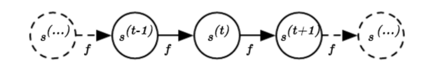

A more generalized form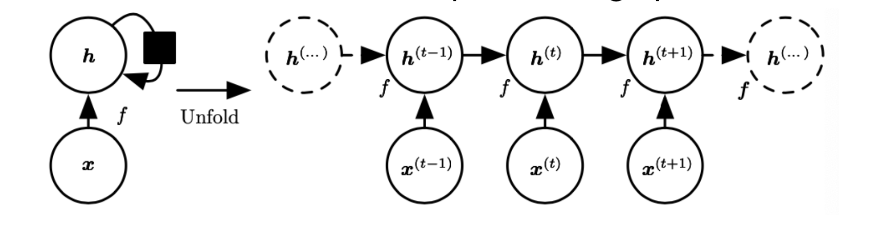

A recurrent neuron with a scalar output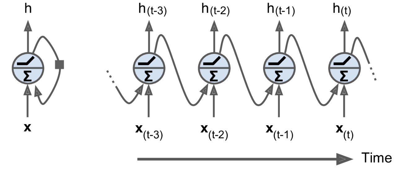

A layer of recurrent neurons with a vector output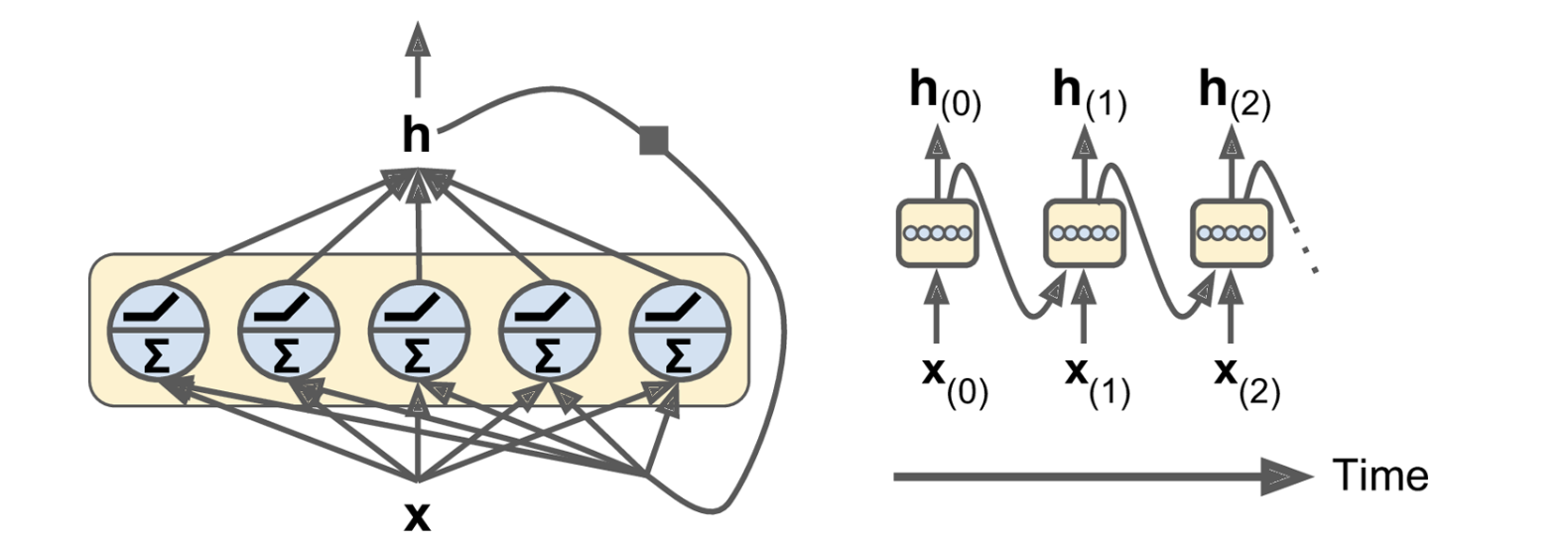

The following gradients (used by gradient-based techniques) can be computed
recursively (details ignored) like the original backpropagation algorithm:

RNN Generalizations

Encoder-Decoder RNN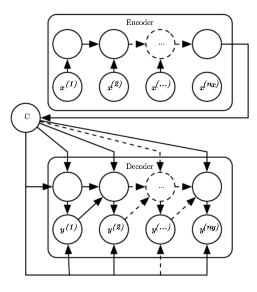

And there are many ways to increase the depth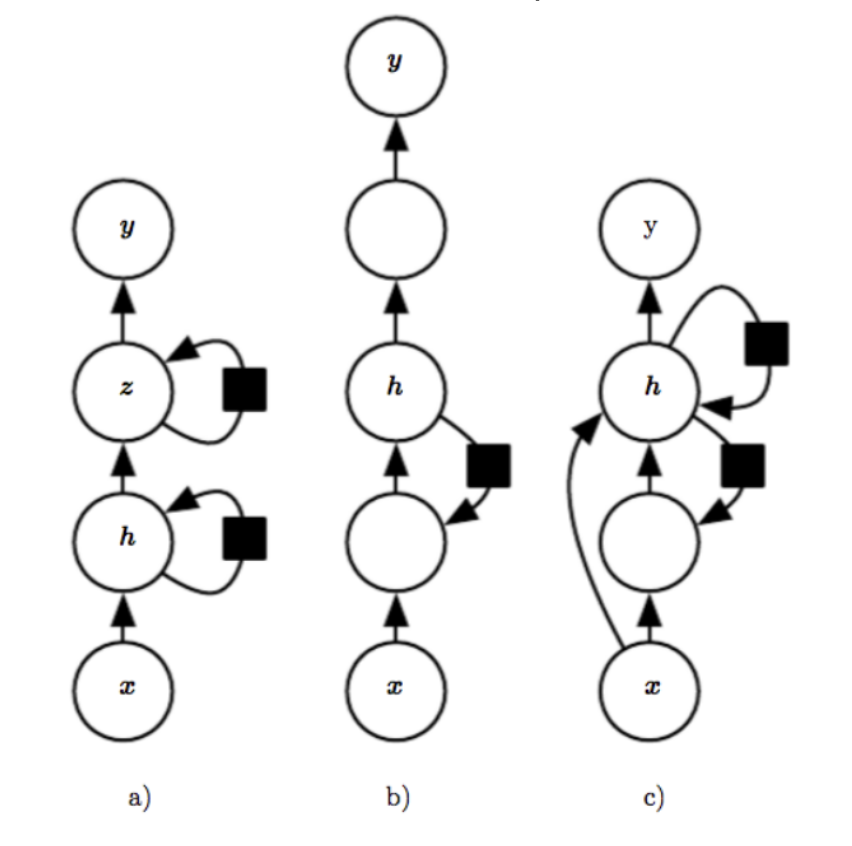

Dependencies between Events in RNNs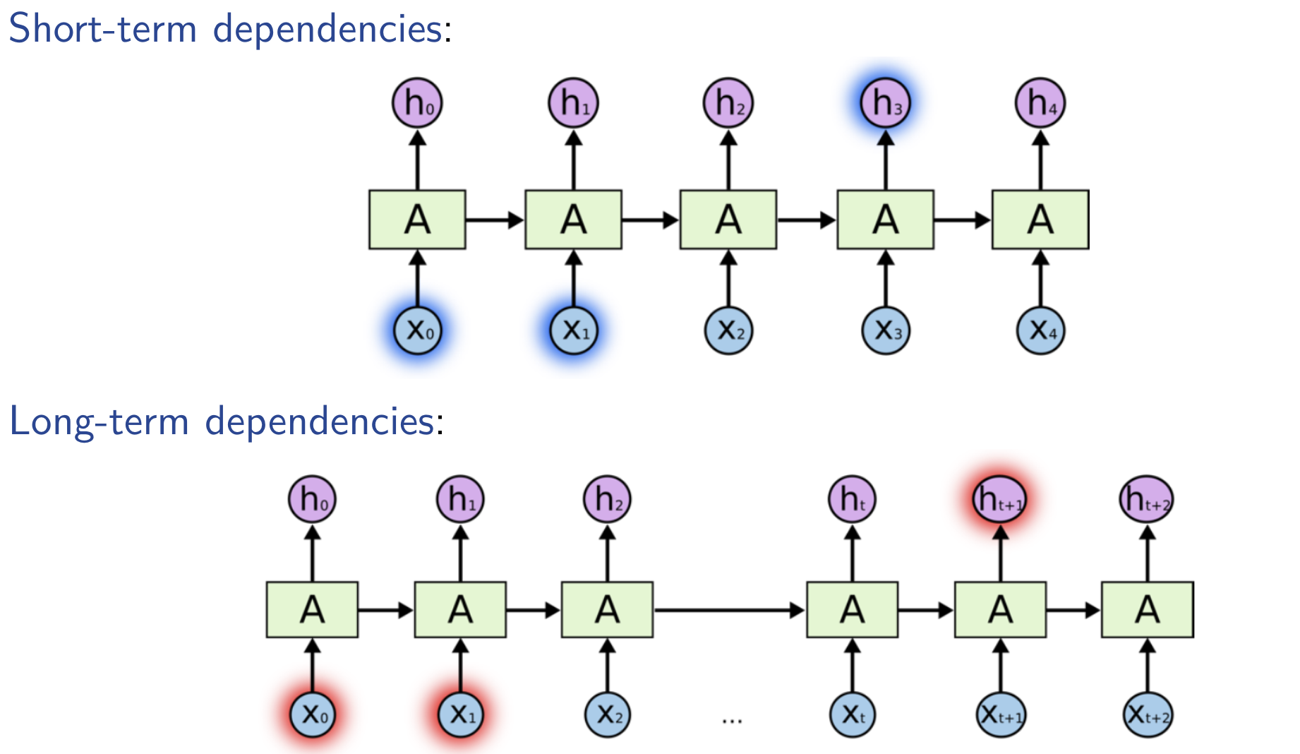

Shortcomings of long-term RNN:1. vanish or explode of gradients.2. computationally intensive
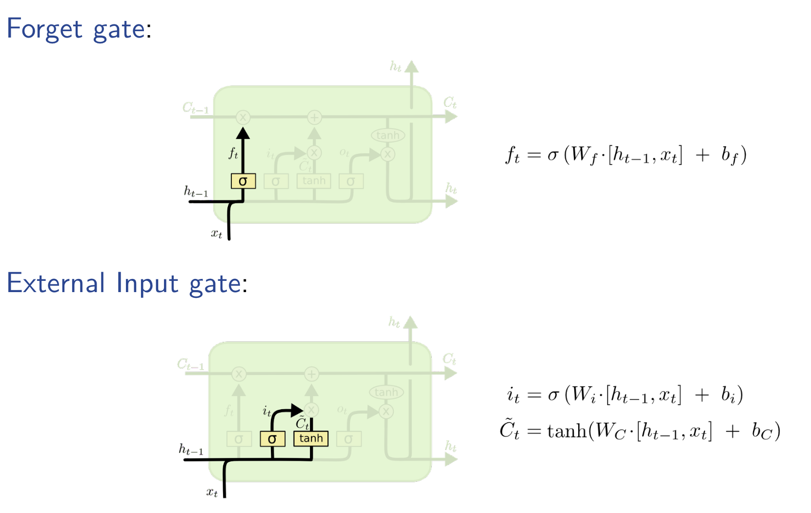
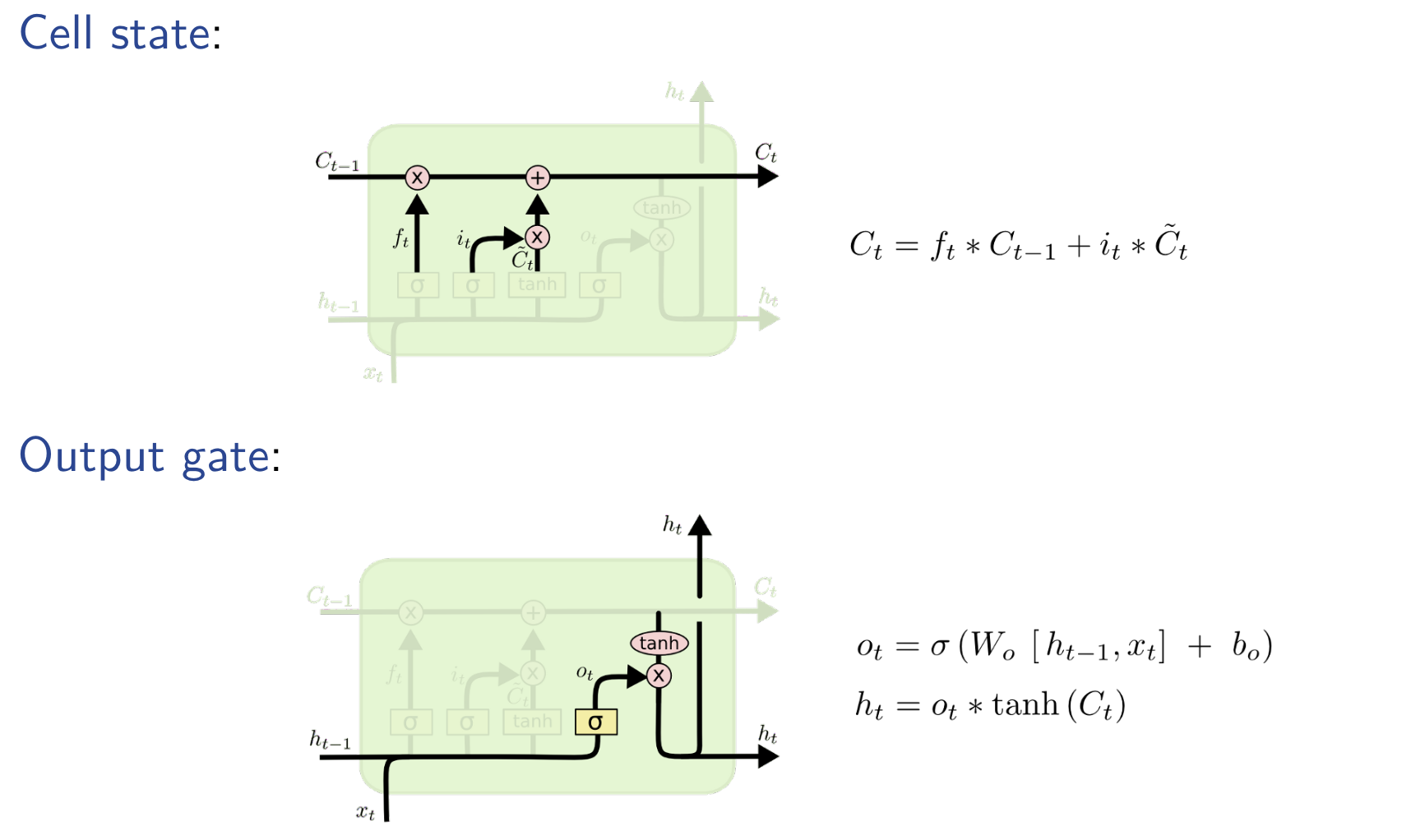
LSTM is based on the idea of leaky units which allow an RNN to accumulateinformation over a longer duration (e.g., we use a leaky unit to accumulate evidence for each subsequence inside a sequence).I Once the information accumulated is used (e.g., suffcient evidence has been accumulated for a subsequence), we need a mechanism to forget the old state by setting it to zero and starting to count again from scratch.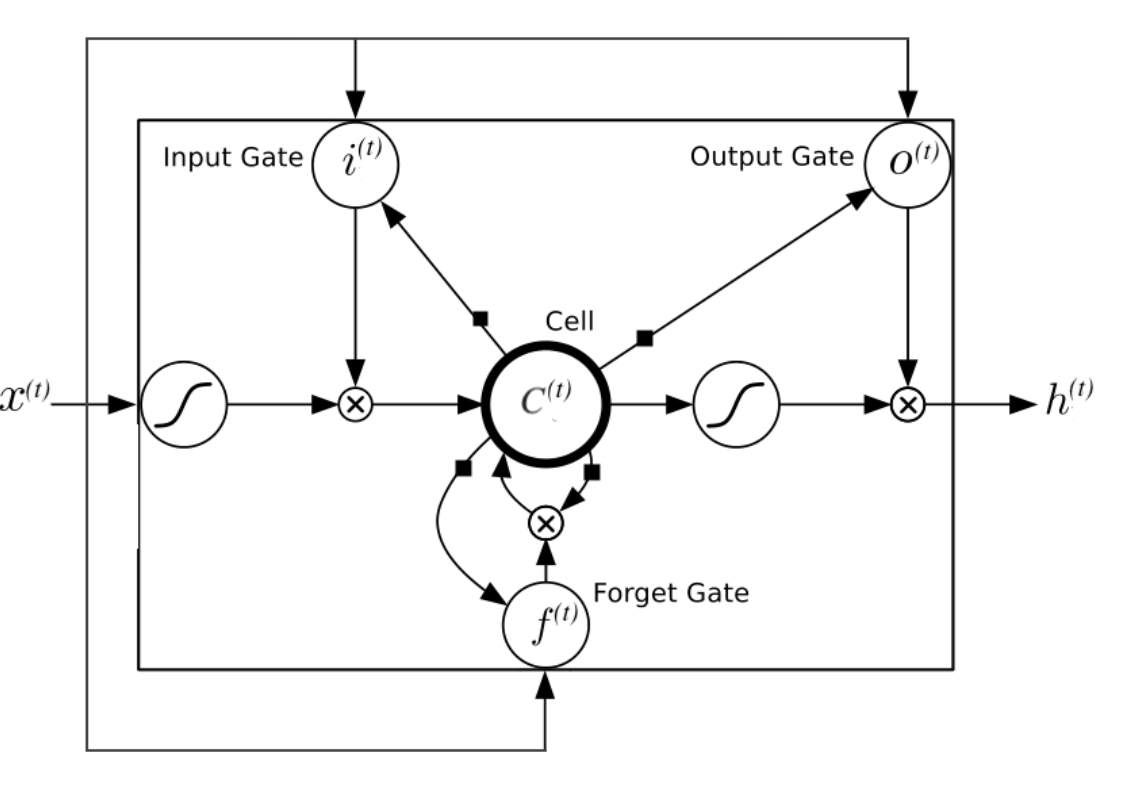

Total RNN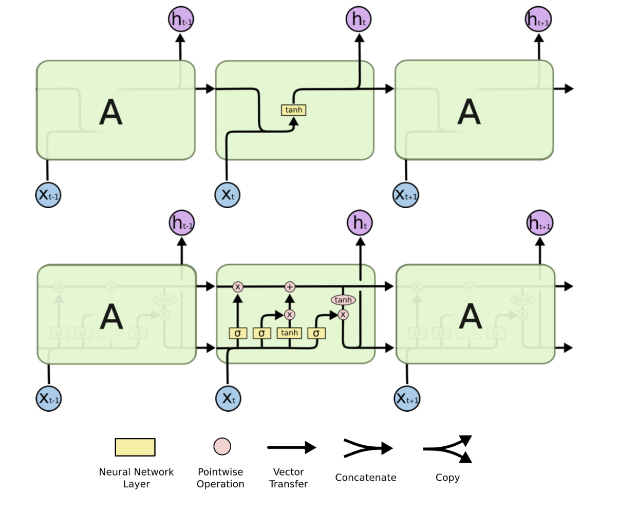

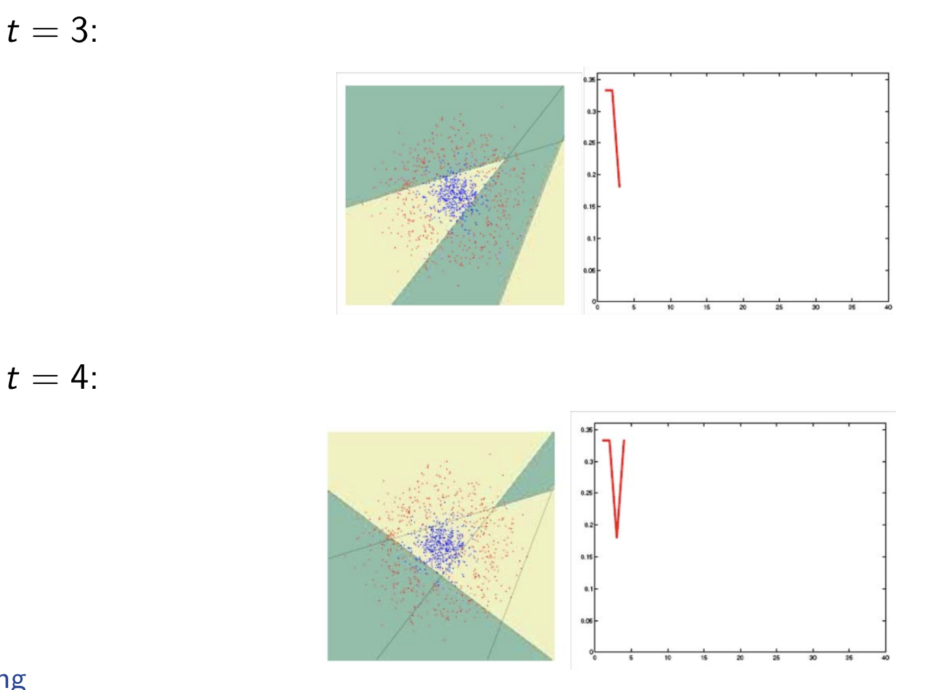
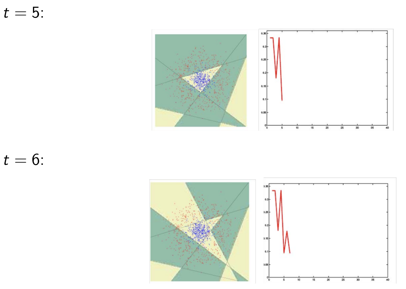
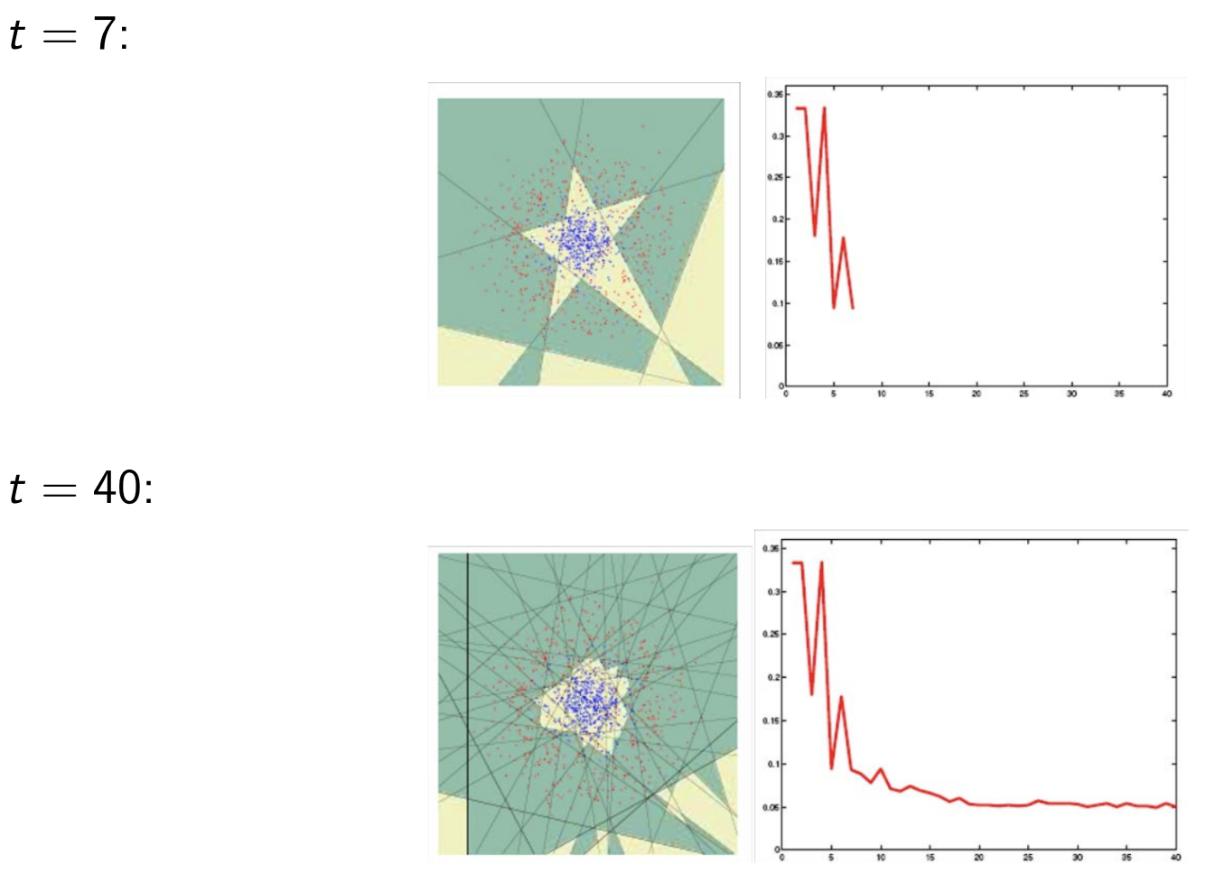
Ensemble Learning

Voting

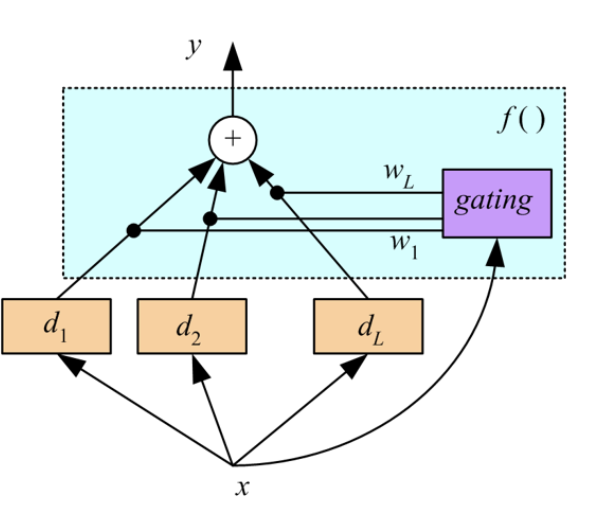
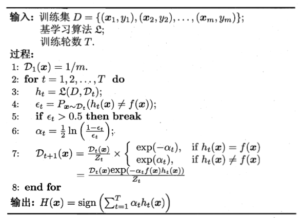
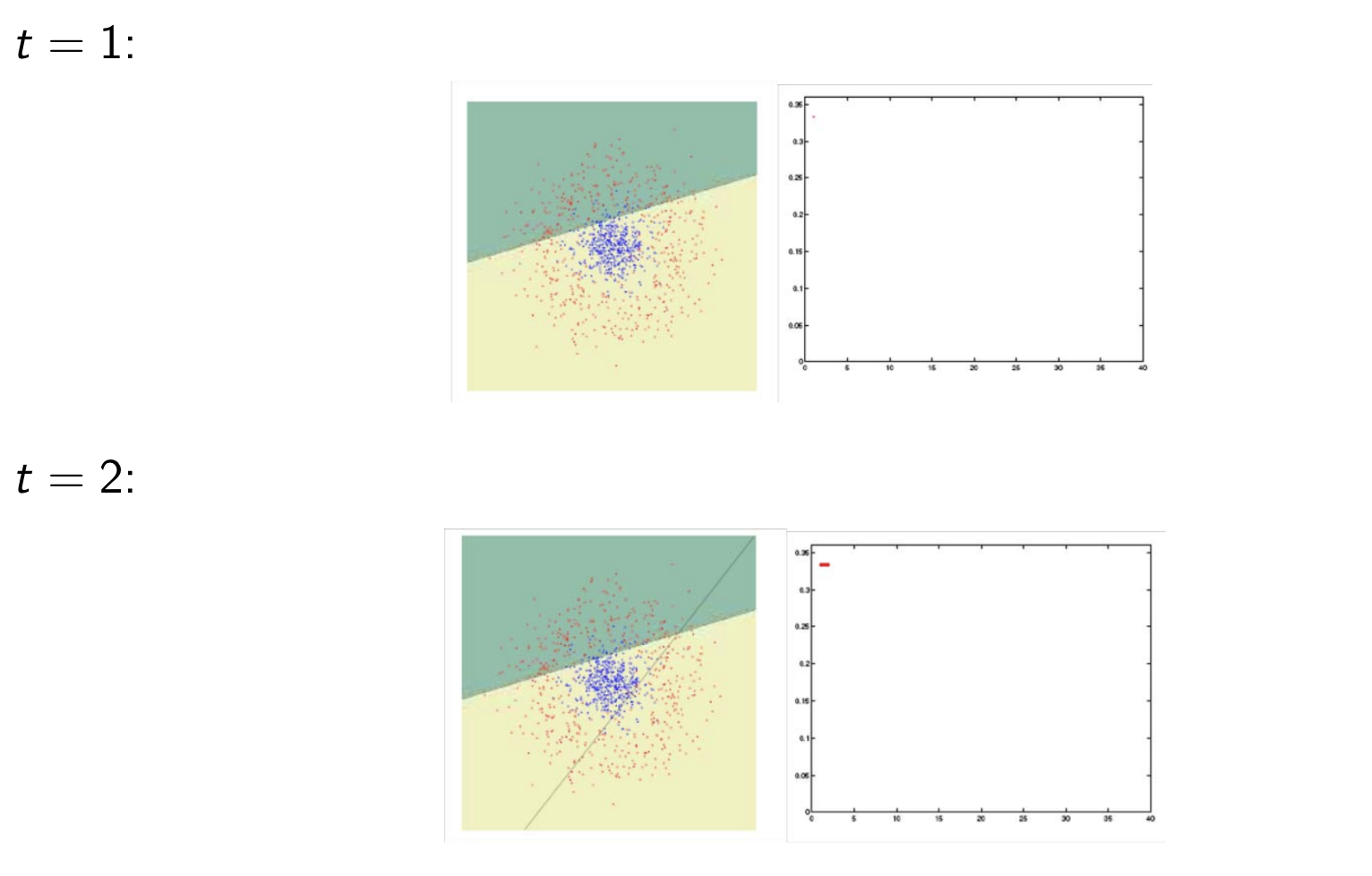
Boosting

Model Assessment Selection

Cross-Validation and Resampling

K-Fold Cross Validation

The datasetis randomly partitioned intoequal-sized subsets,, called folds.

training/validation set pairs:

$$
\begin{aligned}
\mathcal{T}_1 &= \mathcal{X}_2 \cup \mathcal{X}_3 \cup \cdots \cup \mathcal{X}_K & \mathcal{V}_1 &= \mathcal{X}_1 \
\mathcal{T}_2 &= \mathcal{X}_1 \cup \mathcal{X}_3 \cup \cdots \cup \mathcal{X}_K & \mathcal{V}_2 &= \mathcal{X}_2 \
& \vdots & & \vdots \
\mathcal{T}_K &= \mathcal{X}_1 \cup \mathcal{X}2 \cup \cdots \cup \mathcal{X}{K-1} & \mathcal{V}_K &= \mathcal{X}_K \
\end{aligned}
$$

Any two training setsand() sharefolds.

5 × 2-Fold Cross-Validation

For each iteration, the datasetis randomly split into two equal-sized parts,and, which leads to a 2-fold cross-validation. With 5 iterations, we gettraining/validation set pairs:

$$
\begin{aligned}
\mathcal{T}_1 &= \mathcal{X}_1^{(1)} & \mathcal{V}_1 &= \mathcal{X}_1^{(2)} \
\mathcal{T}_2 &= \mathcal{X}_1^{(2)} & \mathcal{V}_2 &= \mathcal{X}_1^{(1)} \
\mathcal{T}_3 &= \mathcal{X}_2^{(1)} & \mathcal{V}_3 &= \mathcal{X}_2^{(2)} \
\mathcal{T}_4 &= \mathcal{X}_2^{(2)} & \mathcal{V}_4 &= \mathcal{X}_2^{(1)} \
& \vdots & & \vdots \
\mathcal{T}_9 &= \mathcal{X}_5^{(1)} & \mathcal{V}_9 &= \mathcal{X}5^{(2)} \
\mathcal{T}{10} &= \mathcal{X}5^{(2)} & \mathcal{V}{10} &= \mathcal{X}_5^{(1)}
\end{aligned}
$$
In total, we have done 5 times of 2-fold cross-validations.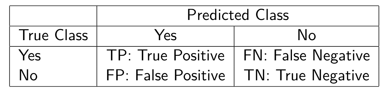

Interval Estimation

Two-sided confidence interval

or

One-sided confidence interval

and

Students’ t-distriburion

In the previous intervals, we used (\sigma); that is, we assumed the variance is known. When the variance (\sigma^2) is not known, it can be replaced by the sample variance

The statisticfollows a t-distribution with (N - 1) degrees of freedom: (long proof omitted here …)

For anywe have used the symmetry around 0 of the t-distribution, i.e.,,

Hypothesis Testing

We can also define a one-sided test or one-tailed test.
Null and alternative hypotheses:

as opposed to the two-sided test when the alternative hypothesis is (\mu \neq \mu_0).
The one-sided test with level of significance (\alpha) defines a 100(1 - (\alpha)) confidence interval bounded on one side in which (m) should lie for the hypothesis not to be rejected.
We fail to reject (H_0) with level of significanceif

Otherwise, we rejectwith region of rejection.
If the varianceis not known, the sample variancewill be used instead and so

E.g., we can define a two-sided t test :

We fail to reject at significance levelif

One-sided t test can be defined similarly.

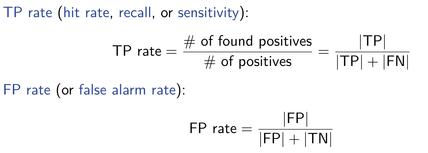
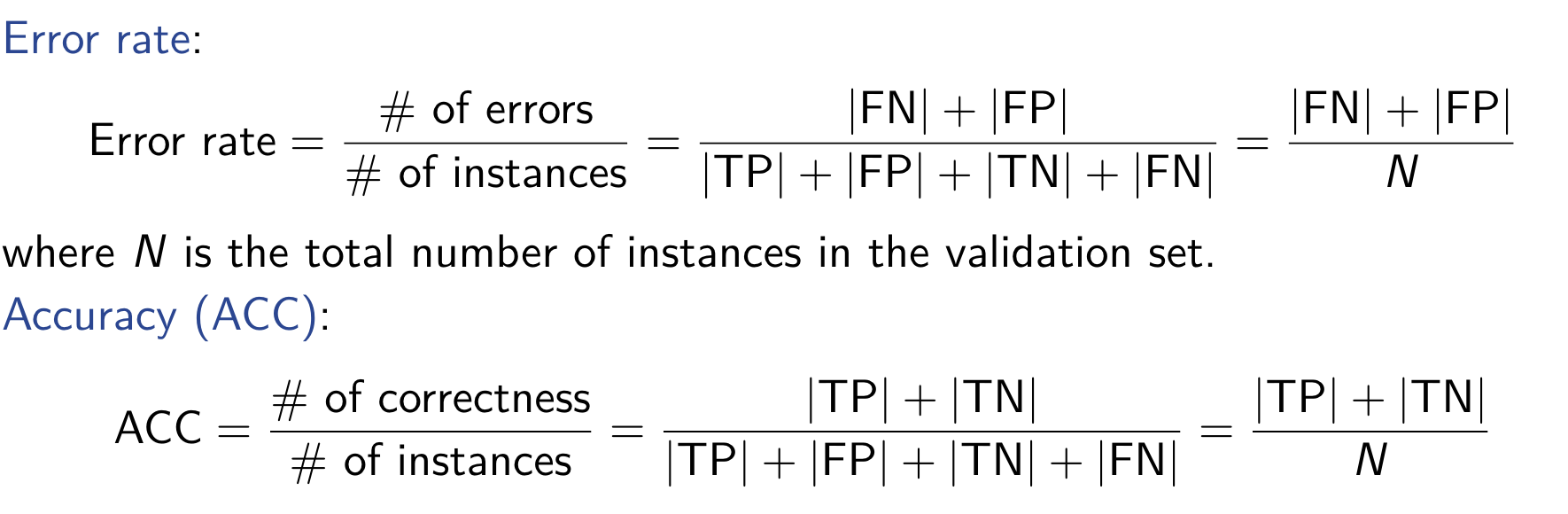
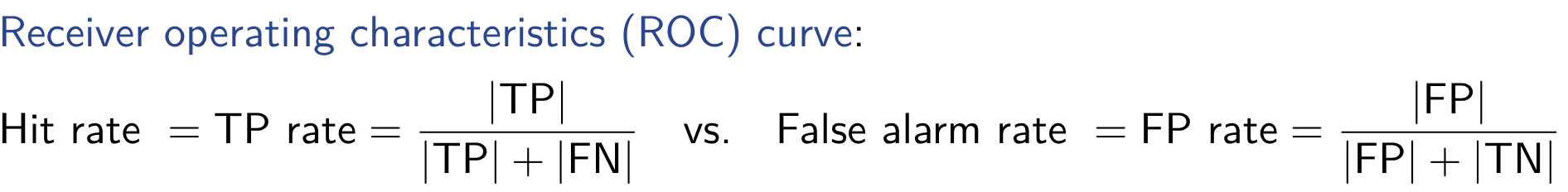
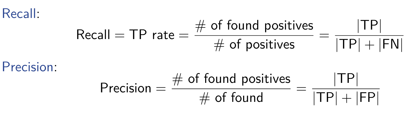
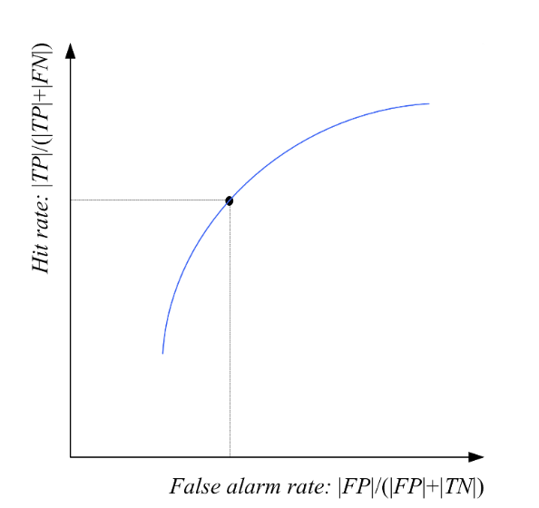
Performance Evaluation

Test statistic: